ホーム » 「MONAI 1.0」タグがついた投稿
タグアーカイブ: MONAI 1.0
MONAI 1.0 : tutorials : 3D セグメンテーション – 脾臓 3D セグメンテーション
MONAI 1.0 : tutorials : 3D セグメンテーション – 脾臓 3D セグメンテーション (翻訳/解説)
翻訳 : (株)クラスキャット セールスインフォメーション
作成日時 : 01/19/2023 (1.1.0)
* 本ページは、MONAI の以下のドキュメントを翻訳した上で適宜、補足説明したものです:
* サンプルコードの動作確認はしておりますが、必要な場合には適宜、追加改変しています。
* ご自由にリンクを張って頂いてかまいませんが、sales-info@classcat.com までご一報いただけると嬉しいです。

- 人工知能研究開発支援
- 人工知能研修サービス(経営者層向けオンサイト研修)
- テクニカルコンサルティングサービス
- 実証実験(プロトタイプ構築)
- アプリケーションへの実装
- 人工知能研修サービス
- PoC(概念実証)を失敗させないための支援
- お住まいの地域に関係なく Web ブラウザからご参加頂けます。事前登録 が必要ですのでご注意ください。
◆ お問合せ : 本件に関するお問い合わせ先は下記までお願いいたします。
- 株式会社クラスキャット セールス・マーケティング本部 セールス・インフォメーション
- sales-info@classcat.com ; Web: www.classcat.com ; ClassCatJP
MONAI 0.7 : tutorials : 3D セグメンテーション – 脾臓 3D セグメンテーション
このノートブックは MSD 脾臓データセット に基づいた 3D セグメンテーションの end-to-end な訓練と評価サンプルです。このサンプルは PyTorch ベースのプログラムで MONAI モジュールの柔軟性を示します :
- 辞書ベースの訓練データ構造のための変換。
- メタデータを含む NIfTI 画像をロードする。
- 想定する範囲で医用画像強度をスケールする。
- ポジティブ/ネガティブ・ラベル比率に基づいてバランスの取れた画像パッチサンプルのバッチをクロップする。
- 訓練と検証を高速化するキャッシュ IO と変換。
- 3D セグメンテーション・タスクのための 3D UNet, Dice 損失関数, Mean Dice メトリック。
- スライディング・ウィンドウ推論。
- 再現性のための決定論的訓練。
このチュートリアルは MONAI を既存の PyTorch 医用 DL プログラムに統合する方法を示します。
そして以下の機能を簡単に使用することができます :
- 辞書形式データのための変換。
- メタデータを含む Nifti 画像をロードする。
- チャネル次元がない場合チャネル dim をデータに追加する。
- 想定される範囲で医用画像強度をスケールする。
- ポジティブ/ネガティブ・ラベル比率に基づいてバランスの取れた画像のバッチをクロップする。
- 訓練と検証を高速化するキャシュ IO と変換。
- 3D セグメンテーション・タスクのための 3D UNet モデル、Dice 損失関数、Mean Dice メトリック。
- スライディング・ウィンドウ推論手法。
- 再現性のための決定論的訓練。
Spleen データセットは http://medicaldecathlon.com/ からダウンロードできます。

- Target: Spleen
- Modality: CT
- Size: 61 3D volumes (41 Training + 20 Testing)
- Source: Memorial Sloan Kettering Cancer Center
- Challenge: Large ranging foreground size
環境のセットアップ
!python -c "import monai" || pip install -q "monai-weekly[gdown, nibabel, tqdm, ignite]"
!python -c "import matplotlib" || pip install -q matplotlib
%matplotlib inline
インポートのセットアップ
from monai.utils import first, set_determinism
from monai.transforms import (
    AsDiscrete,
    AsDiscreted,
    EnsureChannelFirstd,
    Compose,
    CropForegroundd,
    LoadImaged,
    Orientationd,
    RandCropByPosNegLabeld,
    SaveImaged,
    ScaleIntensityRanged,
    Spacingd,
    Invertd,
)
from monai.handlers.utils import from_engine
from monai.networks.nets import UNet
from monai.networks.layers import Norm
from monai.metrics import DiceMetric
from monai.losses import DiceLoss
from monai.inferers import sliding_window_inference
from monai.data import CacheDataset, DataLoader, Dataset, decollate_batch
from monai.config import print_config
from monai.apps import download_and_extract
import torch
import matplotlib.pyplot as plt
import tempfile
import shutil
import os
import glob

print_config()
MONAI version: 1.1.0+2.g97918e46
Numpy version: 1.22.2
Pytorch version: 1.13.0a0+d0d6b1f
MONAI flags: HAS_EXT = True, USE_COMPILED = False, USE_META_DICT = False
MONAI rev id: 97918e46e0d2700c050e678d72e3edb35afbd737
MONAI __file__: /opt/monai/monai/__init__.py

Optional dependencies:
Pytorch Ignite version: 0.4.10
Nibabel version: 4.0.2
scikit-image version: 0.19.3
Pillow version: 9.0.1
Tensorboard version: 2.10.1
gdown version: 4.6.0
TorchVision version: 0.14.0a0
tqdm version: 4.64.1
lmdb version: 1.3.0
psutil version: 5.9.2
pandas version: 1.4.4
einops version: 0.6.0
transformers version: 4.21.3
mlflow version: 2.0.1
pynrrd version: 1.0.0

For details about installing the optional dependencies, please visit:
    https://docs.monai.io/en/latest/installation.html#installing-the-recommended-dependencies
データディレクトリのセットアップ
MONAI_DATA_DIRECTORY 環境変数でディレクトリを指定できます。
これは結果をセーブしてダウンロードを再利用することを可能にします。
指定されない場合、一時ディレクトリが使用されます。
directory = os.environ.get("MONAI_DATA_DIRECTORY")
root_dir = tempfile.mkdtemp() if directory is None else directory
print(root_dir)
/workspace/data/medical/
データセットのダウンロード
データセットをダウンロードして展開します。データセットは http://medicaldecathlon.com/ に由来します。
resource = "https://msd-for-monai.s3-us-west-2.amazonaws.com/Task09_Spleen.tar"
md5 = "410d4a301da4e5b2f6f86ec3ddba524e"

compressed_file = os.path.join(root_dir, "Task09_Spleen.tar")
data_dir = os.path.join(root_dir, "Task09_Spleen")
if not os.path.exists(data_dir):
    download_and_extract(resource, compressed_file, root_dir, md5)
MSD 脾臓データセット・パスの設定
train_images = sorted(
    glob.glob(os.path.join(data_dir, "imagesTr", "*.nii.gz")))
train_labels = sorted(
    glob.glob(os.path.join(data_dir, "labelsTr", "*.nii.gz")))
data_dicts = [
    {"image": image_name, "label": label_name}
    for image_name, label_name in zip(train_images, train_labels)
]
train_files, val_files = data_dicts[:-9], data_dicts[-9:]
再現性のための決定論的訓練の設定
set_determinism(seed=0)
訓練と検証のための変換のセットアップ
ここではデータセットを増強するために幾つかの変換を使用します :
- LoadImaged は NIfTI 形式ファイルから脾臓 CT 画像とラベルをロードします。
- EnsureChannelFirstd は元のデータが「チャネル first」shape を構成することを保証します。
- Orientationd はアフィン行列に基づいてデータの向きを統一します。
- Spacingd はアフィン行列に基づいて pixdim=(1.5, 1.5, 2.) による spacing を調整します。
- ScaleIntensityRanged は強度範囲 [-57, 164] を抽出して [0, 1] にスケールします。
- CropForegroundd は画像とラベルの valid body 領域にフォーカスするために総てのゼロ境界 (= border) を削除します。
- RandCropByPosNegLabeld は pos / neg 比率に基づいて大きな画像からランダムにパッチサンプルをクロップします。
ネガティブサンプルの画像中心は valid body 領域になければなりません。
- RandAffined は PyTorch アフィン変換に基づいて回転, スケール, shear, 並行移動等を一緒に効率的に実行します。
train_transforms = Compose(
    [
        LoadImaged(keys=["image", "label"]),
        EnsureChannelFirstd(keys=["image", "label"]),
        ScaleIntensityRanged(
            keys=["image"], a_min=-57, a_max=164,
            b_min=0.0, b_max=1.0, clip=True,
        ),
        CropForegroundd(keys=["image", "label"], source_key="image"),
        Orientationd(keys=["image", "label"], axcodes="RAS"),
        Spacingd(keys=["image", "label"], pixdim=(
            1.5, 1.5, 2.0), mode=("bilinear", "nearest")),
        RandCropByPosNegLabeld(
            keys=["image", "label"],
            label_key="label",
            spatial_size=(96, 96, 96),
            pos=1,
            neg=1,
            num_samples=4,
            image_key="image",
            image_threshold=0,
        ),
        # user can also add other random transforms
        # RandAffined(
        #     keys=['image', 'label'],
        #     mode=('bilinear', 'nearest'),
        #     prob=1.0, spatial_size=(96, 96, 96),
        #     rotate_range=(0, 0, np.pi/15),
        #     scale_range=(0.1, 0.1, 0.1)),
    ]
)
val_transforms = Compose(
    [
        LoadImaged(keys=["image", "label"]),
        EnsureChannelFirstd(keys=["image", "label"]),
        ScaleIntensityRanged(
            keys=["image"], a_min=-57, a_max=164,
            b_min=0.0, b_max=1.0, clip=True,
        ),
        CropForegroundd(keys=["image", "label"], source_key="image"),
        Orientationd(keys=["image", "label"], axcodes="RAS"),
        Spacingd(keys=["image", "label"], pixdim=(
            1.5, 1.5, 2.0), mode=("bilinear", "nearest")),
    ]
)
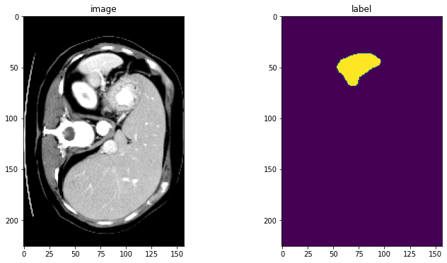
DataLoaer で変換を確認する
check_ds = Dataset(data=val_files, transform=val_transforms)
check_loader = DataLoader(check_ds, batch_size=1)
check_data = first(check_loader)
image, label = (check_data["image"][0][0], check_data["label"][0][0])
print(f"image shape: {image.shape}, label shape: {label.shape}")
# plot the slice [:, :, 80]
plt.figure("check", (12, 6))
plt.subplot(1, 2, 1)
plt.title("image")
plt.imshow(image[:, :, 80], cmap="gray")
plt.subplot(1, 2, 2)
plt.title("label")
plt.imshow(label[:, :, 80])
plt.show()
image shape: torch.Size([226, 157, 113]), label shape: torch.Size([226, 157, 113])
訓練と検証のために CacheDataset と DataLoader を定義する
ここで訓練と検証プロセスを高速化するために CacheDataset を使用し、それは通常の Dataset よりも 10x 高速です。ベストなパフォーマンスを得るためには、総てのデータをキャッシュするために cache_rate=1.0 を設定します、メモリが十分でない場合には、低い値を設定してください。ユーザはまた cache_rate の代わりに cache_num を設定することもできて、2 つの設定の最小値を使用します。そしてキャッシュする間にマルチスレッドを有効にするために num_workers を設定します。通常の Dataset を試したい場合は、下でコメントされたコードを単に使用するように変更してください。
train_ds = CacheDataset(
    data=train_files, transform=train_transforms,
    cache_rate=1.0, num_workers=4)
# train_ds = Dataset(data=train_files, transform=train_transforms)

# use batch_size=2 to load images and use RandCropByPosNegLabeld
# to generate 2 x 4 images for network training
train_loader = DataLoader(train_ds, batch_size=2, shuffle=True, num_workers=4)

val_ds = CacheDataset(
    data=val_files, transform=val_transforms, cache_rate=1.0, num_workers=4)
# val_ds = Dataset(data=val_files, transform=val_transforms)
val_loader = DataLoader(val_ds, batch_size=1, num_workers=4)
Loading dataset: 100%|██████████| 32/32 [00:32<00:00,  1.02s/it]
Loading dataset: 100%|██████████| 9/9 [00:07<00:00,  1.18it/s]
モデル、損失、Optimizer を作成する
# standard PyTorch program style: create UNet, DiceLoss and Adam optimizer
device = torch.device("cuda:0")
model = UNet(
    spatial_dims=3,
    in_channels=1,
    out_channels=2,
    channels=(16, 32, 64, 128, 256),
    strides=(2, 2, 2, 2),
    num_res_units=2,
    norm=Norm.BATCH,
).to(device)
loss_function = DiceLoss(to_onehot_y=True, softmax=True)
optimizer = torch.optim.Adam(model.parameters(), 1e-4)
dice_metric = DiceMetric(include_background=False, reduction="mean")
典型的な PyTorch 訓練プロセスを実行する
max_epochs = 600
val_interval = 2
best_metric = -1
best_metric_epoch = -1
epoch_loss_values = []
metric_values = []
post_pred = Compose([AsDiscrete(argmax=True, to_onehot=2)])
post_label = Compose([AsDiscrete(to_onehot=2)])

for epoch in range(max_epochs):
    print("-" * 10)
    print(f"epoch {epoch + 1}/{max_epochs}")
    model.train()
    epoch_loss = 0
    step = 0
    for batch_data in train_loader:
        step += 1
        inputs, labels = (
            batch_data["image"].to(device),
            batch_data["label"].to(device),
        )
        optimizer.zero_grad()
        outputs = model(inputs)
        loss = loss_function(outputs, labels)
        loss.backward()
        optimizer.step()
        epoch_loss += loss.item()
        print(
            f"{step}/{len(train_ds) // train_loader.batch_size}, "
            f"train_loss: {loss.item():.4f}")
    epoch_loss /= step
    epoch_loss_values.append(epoch_loss)
    print(f"epoch {epoch + 1} average loss: {epoch_loss:.4f}")

    if (epoch + 1) % val_interval == 0:
        model.eval()
        with torch.no_grad():
            for val_data in val_loader:
                val_inputs, val_labels = (
                    val_data["image"].to(device),
                    val_data["label"].to(device),
                )
                roi_size = (160, 160, 160)
                sw_batch_size = 4
                val_outputs = sliding_window_inference(
                    val_inputs, roi_size, sw_batch_size, model)
                val_outputs = [post_pred(i) for i in decollate_batch(val_outputs)]
                val_labels = [post_label(i) for i in decollate_batch(val_labels)]
                # compute metric for current iteration
                dice_metric(y_pred=val_outputs, y=val_labels)

            # aggregate the final mean dice result
            metric = dice_metric.aggregate().item()
            # reset the status for next validation round
            dice_metric.reset()

            metric_values.append(metric)
            if metric > best_metric:
                best_metric = metric
                best_metric_epoch = epoch + 1
                torch.save(model.state_dict(), os.path.join(
                    root_dir, "best_metric_model.pth"))
                print("saved new best metric model")
            print(
                f"current epoch: {epoch + 1} current mean dice: {metric:.4f}"
                f"\nbest mean dice: {best_metric:.4f} "
                f"at epoch: {best_metric_epoch}"
            )
print(
    f"train completed, best_metric: {best_metric:.4f} "
    f"at epoch: {best_metric_epoch}")
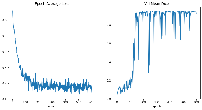
train completed, best_metric: 0.9510 at epoch: 598
損失とメトリックをプロットする
plt.figure("train", (12, 6))
plt.subplot(1, 2, 1)
plt.title("Epoch Average Loss")
x = [i + 1 for i in range(len(epoch_loss_values))]
y = epoch_loss_values
plt.xlabel("epoch")
plt.plot(x, y)
plt.subplot(1, 2, 2)
plt.title("Val Mean Dice")
x = [val_interval * (i + 1) for i in range(len(metric_values))]
y = metric_values
plt.xlabel("epoch")
plt.plot(x, y)
plt.show()
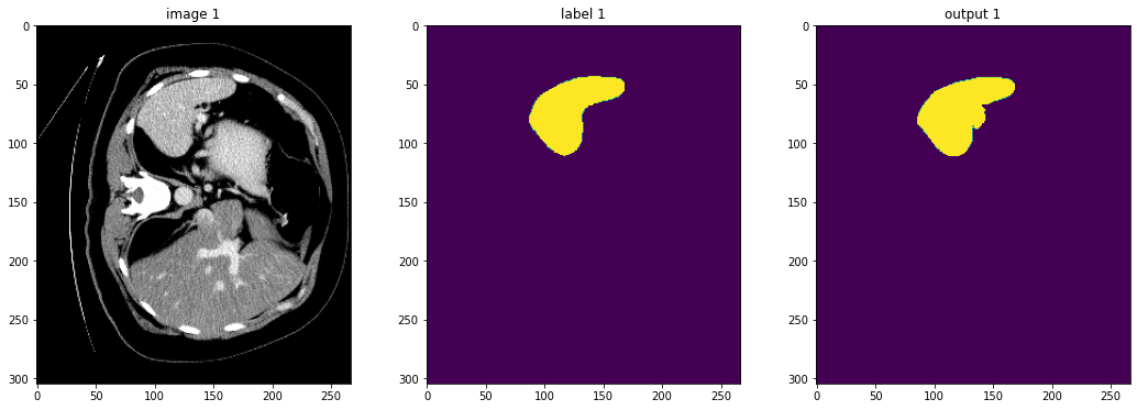
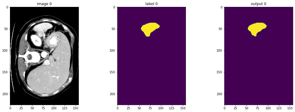
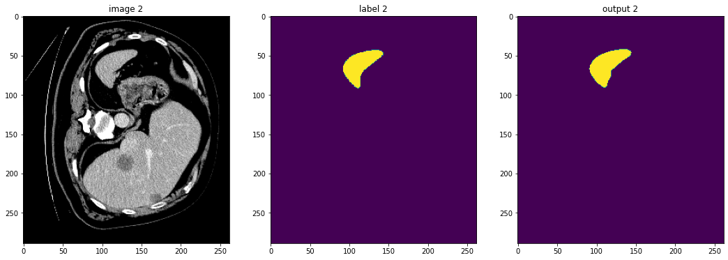
入力画像とラベルでベストなモデル出力を確認する
model.load_state_dict(torch.load(
    os.path.join(root_dir, "best_metric_model.pth")))
model.eval()
with torch.no_grad():
    for i, val_data in enumerate(val_loader):
        roi_size = (160, 160, 160)
        sw_batch_size = 4
        val_outputs = sliding_window_inference(
            val_data["image"].to(device), roi_size, sw_batch_size, model
        )
        # plot the slice [:, :, 80]
        plt.figure("check", (18, 6))
        plt.subplot(1, 3, 1)
        plt.title(f"image {i}")
        plt.imshow(val_data["image"][0, 0, :, :, 80], cmap="gray")
        plt.subplot(1, 3, 2)
        plt.title(f"label {i}")
        plt.imshow(val_data["label"][0, 0, :, :, 80])
        plt.subplot(1, 3, 3)
        plt.title(f"output {i}")
        plt.imshow(torch.argmax(
            val_outputs, dim=1).detach().cpu()[0, :, :, 80])
        plt.show()
        if i == 2:
            break
元の画像 spacing 上の評価
val_org_transforms = Compose(
    [
        LoadImaged(keys=["image", "label"]),
        EnsureChannelFirstd(keys=["image", "label"]),
        Orientationd(keys=["image"], axcodes="RAS"),
        Spacingd(keys=["image"], pixdim=(
            1.5, 1.5, 2.0), mode="bilinear"),
        ScaleIntensityRanged(
            keys=["image"], a_min=-57, a_max=164,
            b_min=0.0, b_max=1.0, clip=True,
        ),
        CropForegroundd(keys=["image"], source_key="image"),
    ]
)

val_org_ds = Dataset(
    data=val_files, transform=val_org_transforms)
val_org_loader = DataLoader(val_org_ds, batch_size=1, num_workers=4)

post_transforms = Compose([
    Invertd(
        keys="pred",
        transform=val_org_transforms,
        orig_keys="image",
        meta_keys="pred_meta_dict",
        orig_meta_keys="image_meta_dict",
        meta_key_postfix="meta_dict",
        nearest_interp=False,
        to_tensor=True,
        device="cpu",
    ),
    AsDiscreted(keys="pred", argmax=True, to_onehot=2),
    AsDiscreted(keys="label", to_onehot=2),
])
model.load_state_dict(torch.load(
    os.path.join(root_dir, "best_metric_model.pth")))
model.eval()

with torch.no_grad():
    for val_data in val_org_loader:
        val_inputs = val_data["image"].to(device)
        roi_size = (160, 160, 160)
        sw_batch_size = 4
        val_data["pred"] = sliding_window_inference(
            val_inputs, roi_size, sw_batch_size, model)
        val_data = [post_transforms(i) for i in decollate_batch(val_data)]
        val_outputs, val_labels = from_engine(["pred", "label"])(val_data)
        # compute metric for current iteration
        dice_metric(y_pred=val_outputs, y=val_labels)

    # aggregate the final mean dice result
    metric_org = dice_metric.aggregate().item()
    # reset the status for next validation round
    dice_metric.reset()

print("Metric on original image spacing: ", metric_org)
Metric on original image spacing: 0.9637420177459717
テストセット上の推論
test_images = sorted(
    glob.glob(os.path.join(data_dir, "imagesTs", "*.nii.gz")))

test_data = [{"image": image} for image in test_images]


test_org_transforms = Compose(
    [
        LoadImaged(keys="image"),
        EnsureChannelFirstd(keys="image"),
        Orientationd(keys=["image"], axcodes="RAS"),
        Spacingd(keys=["image"], pixdim=(
            1.5, 1.5, 2.0), mode="bilinear"),
        ScaleIntensityRanged(
            keys=["image"], a_min=-57, a_max=164,
            b_min=0.0, b_max=1.0, clip=True,
        ),
        CropForegroundd(keys=["image"], source_key="image"),
    ]
)

test_org_ds = Dataset(
    data=test_data, transform=test_org_transforms)

test_org_loader = DataLoader(test_org_ds, batch_size=1, num_workers=4)

post_transforms = Compose([
    Invertd(
        keys="pred",
        transform=test_org_transforms,
        orig_keys="image",
        meta_keys="pred_meta_dict",
        orig_meta_keys="image_meta_dict",
        meta_key_postfix="meta_dict",
        nearest_interp=False,
        to_tensor=True,
    ),
    AsDiscreted(keys="pred", argmax=True, to_onehot=2),
    SaveImaged(keys="pred", meta_keys="pred_meta_dict", output_dir="./out", output_postfix="seg", resample=False),
])
# # uncomment the following lines to visualize the predicted results
# from monai.transforms import LoadImage
# loader = LoadImage()
model.load_state_dict(torch.load(
    os.path.join(root_dir, "best_metric_model.pth")))
model.eval()

with torch.no_grad():
    for test_data in test_org_loader:
        test_inputs = test_data["image"].to(device)
        roi_size = (160, 160, 160)
        sw_batch_size = 4
        test_data["pred"] = sliding_window_inference(
            test_inputs, roi_size, sw_batch_size, model)

        test_data = [post_transforms(i) for i in decollate_batch(test_data)]

#         # uncomment the following lines to visualize the predicted results
#         test_output = from_engine(["pred"])(test_data)

#         original_image = loader(test_output[0].meta["filename_or_obj"])

#         plt.figure("check", (18, 6))
#         plt.subplot(1, 2, 1)
#         plt.imshow(original_image[:, :, 20], cmap="gray")
#         plt.subplot(1, 2, 2)
#         plt.imshow(test_output[0].detach().cpu()[1, :, :, 20])
#         plt.show()
データディレクトリのクリーンアップ
一時ディレクトリが使用された場合にはディレクトリを削除します。
if directory is None:
    shutil.rmtree(root_dir)
以上
MONAI 1.0 : tutorials : 3D セグメンテーション – 脳腫瘍 3D セグメンテーション
MONAI 1.0 : tutorials : 3D セグメンテーション – 脳腫瘍 3D セグメンテーション (翻訳/解説)
翻訳 : (株)クラスキャット セールスインフォメーション
作成日時 : 01/18/2023 (1.1.0)
* 本ページは、MONAI の以下のドキュメントを翻訳した上で適宜、補足説明したものです:
* サンプルコードの動作確認はしておりますが、必要な場合には適宜、追加改変しています。
* ご自由にリンクを張って頂いてかまいませんが、sales-info@classcat.com までご一報いただけると嬉しいです。
- 人工知能研究開発支援
- 人工知能研修サービス(経営者層向けオンサイト研修)
- テクニカルコンサルティングサービス
- 実証実験(プロトタイプ構築)
- アプリケーションへの実装
- 人工知能研修サービス
- PoC(概念実証)を失敗させないための支援
- お住まいの地域に関係なく Web ブラウザからご参加頂けます。事前登録 が必要ですのでご注意ください。
◆ お問合せ : 本件に関するお問い合わせ先は下記までお願いいたします。
- 株式会社クラスキャット セールス・マーケティング本部 セールス・インフォメーション
- sales-info@classcat.com ; Web: www.classcat.com ; ClassCatJP
MONAI 1.0 : tutorials : 3D セグメンテーション – 脳腫瘍 3D セグメンテーション
このチュートリアルは MSD 脳腫瘍データセット に基づくマルチラベル・セグメンテーションタスクの訓練ワークフローを構築する方法を示します。
このチュートリアルはマルチラベル・セグメンテーション・タスクの訓練ワークフローを構築する方法を示します。
そしてそれは以下の機能を含みます :
- 辞書形式データ用の変換。
- MONAI 変換 API に従って新しい変換を定義する。
- メタデータと共に Nifti 画像をロードし、画像のリストをロードしてそれらをスタックする。
- データ増強のために強度をランダムに調整する。
- 訓練と検証を高速化する Cache IO と変換。
- 3D セグメンテーション・タスクのための 3D SegResNet モデル, Dice 損失関数, 平均 Dice メトリック。
- 再現性のための決定論的訓練。
データセットは http://medicaldecathlon.com/ に由来します。
ターゲット: Gliomas segmentation necrotic/active tumour and oedema
モダリティ: マルチモーダル multisite MRI データ (FLAIR, T1w, T1gd,T2w)
サイズ: 750 4D ボリューム (484 訓練 + 266 テスト)
ソース: BRATS 2016 と 2017 データセット。
チャレンジ: Complex and heterogeneously-located targets
下図は、様々なモダリティでアノテートされている腫瘍部分領域の画像パッチ (左上) とデータセット全体のための最終的なラベル (右) を示します。(図は BraTS IEEE TMI 論文 から引用)
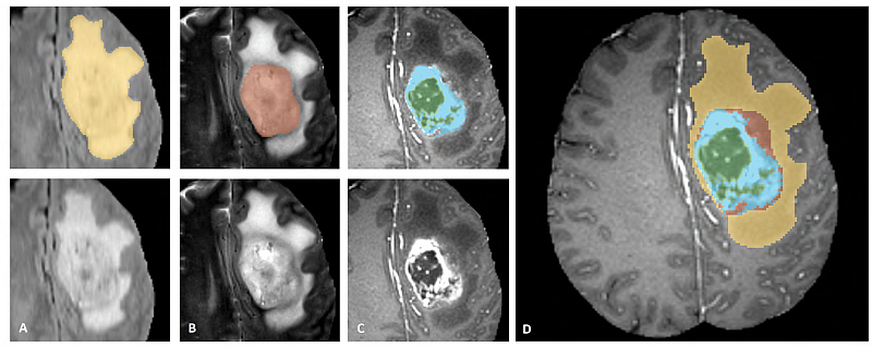
画像パッチは左から右へ以下を示します :
- T2-FLAIR で見える腫瘍全体 (黄色) (Fig.A)。
- T2 で見える腫瘍のコア (赤色) (Fig. B)。
- T1Gd で見える enhancing 腫瘍構造 (ライトブルー)、これはコアの嚢胞 (のうほう) (= cystic) / 壊死 (=necrotic) 成分 (緑色) を取り囲んでいます (Fig. C)。
- セグメンテーションは 腫瘍部分領域の最終的なラベル (Fig.D) を生成するために組み合わされます : 浮腫 (= edema) (黄色), non-enhancing ソリッドコア (赤色), 嚢胞/壊死コア (緑色), enhancing コア (青色) です。
環境のセットアップ
!python -c "import monai" || pip install -q "monai-weekly[nibabel, tqdm]"
!python -c "import matplotlib" || pip install -q matplotlib
%matplotlib inline
インポートのセットアップ
import os
import shutil
import tempfile
import time
import matplotlib.pyplot as plt
from monai.apps import DecathlonDataset
from monai.config import print_config
from monai.data import DataLoader, decollate_batch
from monai.handlers.utils import from_engine
from monai.losses import DiceLoss
from monai.inferers import sliding_window_inference
from monai.metrics import DiceMetric
from monai.networks.nets import SegResNet
from monai.transforms import (
    Activations,
    Activationsd,
    AsDiscrete,
    AsDiscreted,
    Compose,
    Invertd,
    LoadImaged,
    MapTransform,
    NormalizeIntensityd,
    Orientationd,
    RandFlipd,
    RandScaleIntensityd,
    RandShiftIntensityd,
    RandSpatialCropd,
    Spacingd,
    EnsureTyped,
    EnsureChannelFirstd,
)
from monai.utils import set_determinism

import torch

print_config()
MONAI version: 0.9.1
Numpy version: 1.22.4
Pytorch version: 1.13.0a0+340c412
MONAI flags: HAS_EXT = True, USE_COMPILED = False, USE_META_DICT = False
MONAI rev id: 356d2d2f41b473f588899d705bbc682308cee52c
MONAI __file__: /opt/monai/monai/__init__.py

Optional dependencies:
Pytorch Ignite version: 0.4.9
Nibabel version: 4.0.1
scikit-image version: 0.19.3
Pillow version: 9.0.1
Tensorboard version: 2.9.1
gdown version: 4.5.1
TorchVision version: 0.13.0a0
tqdm version: 4.64.0
lmdb version: 1.3.0
psutil version: 5.9.1
pandas version: 1.3.5
einops version: 0.4.1
transformers version: 4.20.1
mlflow version: 1.27.0
pynrrd version: 0.4.3

For details about installing the optional dependencies, please visit:
    https://docs.monai.io/en/latest/installation.html#installing-the-recommended-dependencies
データディレクトリのセットアップ
MONAI_DATA_DIRECTORY 環境変数でディレクトリを指定できます。これは結果をセーブしてダウンロードを再利用することを可能にします。指定されない場合、一時ディレクトリが使用されます。
directory = os.environ.get("MONAI_DATA_DIRECTORY")
root_dir = tempfile.mkdtemp() if directory is None else directory
print(root_dir)
/workspace/data/medical
再現性のために決定論的訓練を設定する
set_determinism(seed=0)
脳腫瘍のラベルを変換するために新しい変換を定義する
ここでは多クラスラベルを One-Hot 形式のマルチラベルのセグメンテーション・タスクに変換します。
class ConvertToMultiChannelBasedOnBratsClassesd(MapTransform):
    """
    Convert labels to multi channels based on brats classes:
    label 1 is the peritumoral edema
    label 2 is the GD-enhancing tumor
    label 3 is the necrotic and non-enhancing tumor core
    The possible classes are TC (Tumor core), WT (Whole tumor)
    and ET (Enhancing tumor).

    """

    def __call__(self, data):
        d = dict(data)
        for key in self.keys:
            result = []
            # merge label 2 and label 3 to construct TC
            result.append(torch.logical_or(d[key] == 2, d[key] == 3))
            # merge labels 1, 2 and 3 to construct WT
            result.append(
                torch.logical_or(
                    torch.logical_or(d[key] == 2, d[key] == 3), d[key] == 1
                )
            )
            # label 2 is ET
            result.append(d[key] == 2)
            d[key] = torch.stack(result, axis=0).float()
        return d
訓練と検証のための変換のセットアップ
train_transform = Compose(
    [
        # load 4 Nifti images and stack them together
        LoadImaged(keys=["image", "label"]),
        EnsureChannelFirstd(keys="image"),
        EnsureTyped(keys=["image", "label"]),
        ConvertToMultiChannelBasedOnBratsClassesd(keys="label"),
        Orientationd(keys=["image", "label"], axcodes="RAS"),
        Spacingd(
            keys=["image", "label"],
            pixdim=(1.0, 1.0, 1.0),
            mode=("bilinear", "nearest"),
        ),
        RandSpatialCropd(keys=["image", "label"], roi_size=[224, 224, 144], random_size=False),
        RandFlipd(keys=["image", "label"], prob=0.5, spatial_axis=0),
        RandFlipd(keys=["image", "label"], prob=0.5, spatial_axis=1),
        RandFlipd(keys=["image", "label"], prob=0.5, spatial_axis=2),
        NormalizeIntensityd(keys="image", nonzero=True, channel_wise=True),
        RandScaleIntensityd(keys="image", factors=0.1, prob=1.0),
        RandShiftIntensityd(keys="image", offsets=0.1, prob=1.0),
    ]
)
val_transform = Compose(
    [
        LoadImaged(keys=["image", "label"]),
        EnsureChannelFirstd(keys="image"),
        EnsureTyped(keys=["image", "label"]),
        ConvertToMultiChannelBasedOnBratsClassesd(keys="label"),
        Orientationd(keys=["image", "label"], axcodes="RAS"),
        Spacingd(
            keys=["image", "label"],
            pixdim=(1.0, 1.0, 1.0),
            mode=("bilinear", "nearest"),
        ),
        NormalizeIntensityd(keys="image", nonzero=True, channel_wise=True),
    ]
)
DecathlonDataset でデータを素早くロードする
ここではデータセットを自動的にダウンロードして抽出するために DecathlonDataset を使用します。それは MONAI CacheDataset を継承し、より少ないメモリを使用したい場合には、訓練のために N 項目をキャッシュするために cache_num=N を設定して検証のために総ての項目をキャッシュするために default args を使用できます、それはメモリサイズに依存します。
# here we don't cache any data in case out of memory issue
train_ds = DecathlonDataset(
    root_dir=root_dir,
    task="Task01_BrainTumour",
    transform=train_transform,
    section="training",
    download=True,
    cache_rate=0.0,
    num_workers=4,
)
train_loader = DataLoader(train_ds, batch_size=1, shuffle=True, num_workers=4)
val_ds = DecathlonDataset(
    root_dir=root_dir,
    task="Task01_BrainTumour",
    transform=val_transform,
    section="validation",
    download=False,
    cache_rate=0.0,
    num_workers=4,
)
val_loader = DataLoader(val_ds, batch_size=1, shuffle=False, num_workers=4)
Verified 'Task01_BrainTumour.tar', md5: 240a19d752f0d9e9101544901065d872.
File exists: /workspace/data/medical/Task01_BrainTumour.tar, skipped downloading.
Non-empty folder exists in /workspace/data/medical/Task01_BrainTumour, skipped extracting.
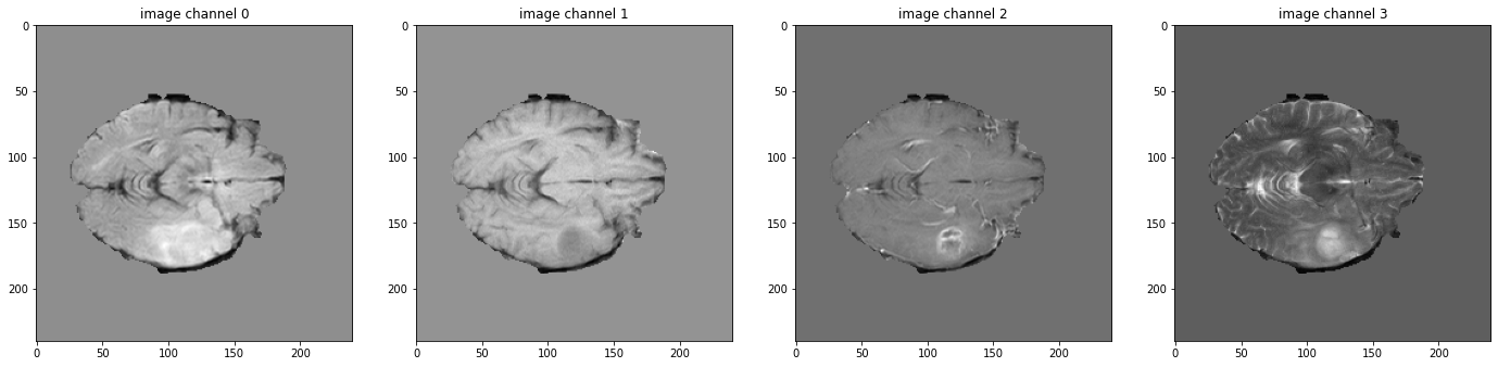
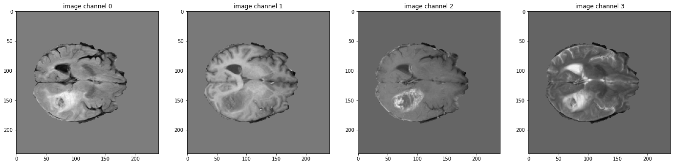
データ shape を確認して可視化する
# pick one image from DecathlonDataset to visualize and check the 4 channels
val_data_example = val_ds[2]
print(f"image shape: {val_data_example['image'].shape}")
plt.figure("image", (24, 6))
for i in range(4):
plt.subplot(1, 4, i + 1)
plt.title(f"image channel {i}")
plt.imshow(val_data_example["image"][i, :, :, 60].detach().cpu(), cmap="gray")
plt.show()
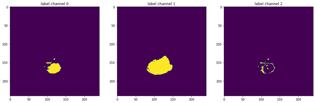
# also visualize the 3 channels label corresponding to this image
print(f"label shape: {val_data_example['label'].shape}")
plt.figure("label", (18, 6))
for i in range(3):
plt.subplot(1, 3, i + 1)
plt.title(f"label channel {i}")
plt.imshow(val_data_example["label"][i, :, :, 60].detach().cpu())
plt.show()
image shape: torch.Size([4, 240, 240, 155])
モデル, 損失, Optimizer を作成する
max_epochs = 300
val_interval = 1
VAL_AMP = True

# standard PyTorch program style: create SegResNet, DiceLoss and Adam optimizer
device = torch.device("cuda:0")
model = SegResNet(
    blocks_down=[1, 2, 2, 4],
    blocks_up=[1, 1, 1],
    init_filters=16,
    in_channels=4,
    out_channels=3,
    dropout_prob=0.2,
).to(device)
loss_function = DiceLoss(smooth_nr=0, smooth_dr=1e-5, squared_pred=True, to_onehot_y=False, sigmoid=True)
optimizer = torch.optim.Adam(model.parameters(), 1e-4, weight_decay=1e-5)
lr_scheduler = torch.optim.lr_scheduler.CosineAnnealingLR(optimizer, T_max=max_epochs)

dice_metric = DiceMetric(include_background=True, reduction="mean")
dice_metric_batch = DiceMetric(include_background=True, reduction="mean_batch")

post_trans = Compose(
    [Activations(sigmoid=True), AsDiscrete(threshold=0.5)]
)


# define inference method
def inference(input):

    def _compute(input):
        return sliding_window_inference(
            inputs=input,
            roi_size=(240, 240, 160),
            sw_batch_size=1,
            predictor=model,
            overlap=0.5,
        )

    if VAL_AMP:
        with torch.cuda.amp.autocast():
            return _compute(input)
    else:
        return _compute(input)


# use amp to accelerate training
scaler = torch.cuda.amp.GradScaler()
# enable cuDNN benchmark
torch.backends.cudnn.benchmark = True
典型的な PyTorch 訓練プロセスの実行
best_metric = -1
best_metric_epoch = -1
best_metrics_epochs_and_time = [[], [], []]
epoch_loss_values = []
metric_values = []
metric_values_tc = []
metric_values_wt = []
metric_values_et = []

total_start = time.time()
for epoch in range(max_epochs):
    epoch_start = time.time()
    print("-" * 10)
    print(f"epoch {epoch + 1}/{max_epochs}")
    model.train()
    epoch_loss = 0
    step = 0
    for batch_data in train_loader:
        step_start = time.time()
        step += 1
        inputs, labels = (
            batch_data["image"].to(device),
            batch_data["label"].to(device),
        )
        optimizer.zero_grad()
        with torch.cuda.amp.autocast():
            outputs = model(inputs)
            loss = loss_function(outputs, labels)
        scaler.scale(loss).backward()
        scaler.step(optimizer)
        scaler.update()
        epoch_loss += loss.item()
        print(
            f"{step}/{len(train_ds) // train_loader.batch_size}"
            f", train_loss: {loss.item():.4f}"
            f", step time: {(time.time() - step_start):.4f}"
        )
    lr_scheduler.step()
    epoch_loss /= step
    epoch_loss_values.append(epoch_loss)
    print(f"epoch {epoch + 1} average loss: {epoch_loss:.4f}")

    if (epoch + 1) % val_interval == 0:
        model.eval()
        with torch.no_grad():

            for val_data in val_loader:
                val_inputs, val_labels = (
                    val_data["image"].to(device),
                    val_data["label"].to(device),
                )
                val_outputs = inference(val_inputs)
                val_outputs = [post_trans(i) for i in decollate_batch(val_outputs)]
                dice_metric(y_pred=val_outputs, y=val_labels)
                dice_metric_batch(y_pred=val_outputs, y=val_labels)

            metric = dice_metric.aggregate().item()
            metric_values.append(metric)
            metric_batch = dice_metric_batch.aggregate()
            metric_tc = metric_batch[0].item()
            metric_values_tc.append(metric_tc)
            metric_wt = metric_batch[1].item()
            metric_values_wt.append(metric_wt)
            metric_et = metric_batch[2].item()
            metric_values_et.append(metric_et)
            dice_metric.reset()
            dice_metric_batch.reset()

            if metric > best_metric:
                best_metric = metric
                best_metric_epoch = epoch + 1
                best_metrics_epochs_and_time[0].append(best_metric)
                best_metrics_epochs_and_time[1].append(best_metric_epoch)
                best_metrics_epochs_and_time[2].append(time.time() - total_start)
                torch.save(
                    model.state_dict(),
                    os.path.join(root_dir, "best_metric_model.pth"),
                )
                print("saved new best metric model")
            print(
                f"current epoch: {epoch + 1} current mean dice: {metric:.4f}"
                f" tc: {metric_tc:.4f} wt: {metric_wt:.4f} et: {metric_et:.4f}"
                f"\nbest mean dice: {best_metric:.4f}"
                f" at epoch: {best_metric_epoch}"
            )
    print(f"time consuming of epoch {epoch + 1} is: {(time.time() - epoch_start):.4f}")
total_time = time.time() - total_start
print(f"train completed, best_metric: {best_metric:.4f} at epoch: {best_metric_epoch}, total time: {total_time}.")
train completed, best_metric: 0.7914 at epoch: 279, total time: 90155.70936012268.
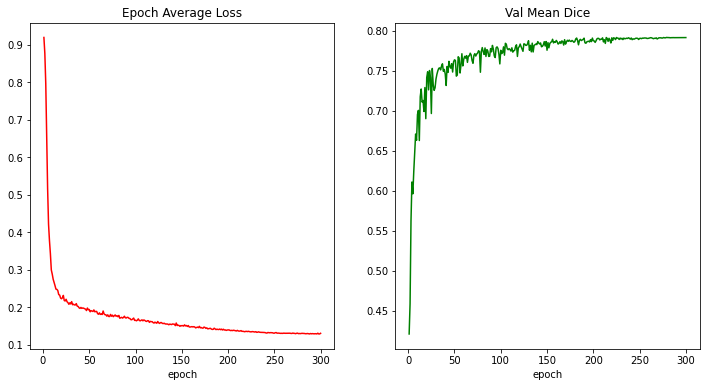
損失とメトリックのプロット
plt.figure("train", (12, 6))
plt.subplot(1, 2, 1)
plt.title("Epoch Average Loss")
x = [i + 1 for i in range(len(epoch_loss_values))]
y = epoch_loss_values
plt.xlabel("epoch")
plt.plot(x, y, color="red")
plt.subplot(1, 2, 2)
plt.title("Val Mean Dice")
x = [val_interval * (i + 1) for i in range(len(metric_values))]
y = metric_values
plt.xlabel("epoch")
plt.plot(x, y, color="green")
plt.show()
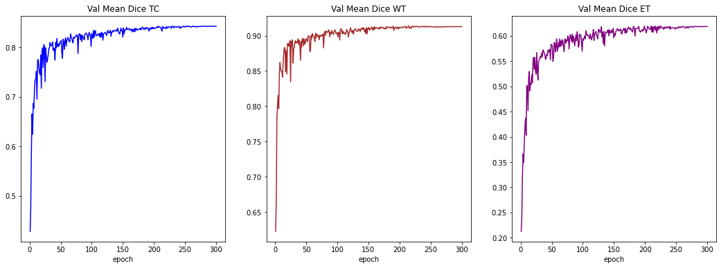
plt.figure("train", (18, 6))
plt.subplot(1, 3, 1)
plt.title("Val Mean Dice TC")
x = [val_interval * (i + 1) for i in range(len(metric_values_tc))]
y = metric_values_tc
plt.xlabel("epoch")
plt.plot(x, y, color="blue")
plt.subplot(1, 3, 2)
plt.title("Val Mean Dice WT")
x = [val_interval * (i + 1) for i in range(len(metric_values_wt))]
y = metric_values_wt
plt.xlabel("epoch")
plt.plot(x, y, color="brown")
plt.subplot(1, 3, 3)
plt.title("Val Mean Dice ET")
x = [val_interval * (i + 1) for i in range(len(metric_values_et))]
y = metric_values_et
plt.xlabel("epoch")
plt.plot(x, y, color="purple")
plt.show()
入力画像とラベルでベストモデル出力を確認する
model.load_state_dict(
torch.load(os.path.join(root_dir, "best_metric_model.pth"))
)
model.eval()
with torch.no_grad():
# select one image to evaluate and visualize the model output
val_input = val_ds[6]["image"].unsqueeze(0).to(device)
roi_size = (128, 128, 64)
sw_batch_size = 4
val_output = inference(val_input)
val_output = post_trans(val_output[0])
plt.figure("image", (24, 6))
for i in range(4):
plt.subplot(1, 4, i + 1)
plt.title(f"image channel {i}")
plt.imshow(val_ds[6]["image"][i, :, :, 70].detach().cpu(), cmap="gray")
plt.show()
# visualize the 3 channels label corresponding to this image
plt.figure("label", (18, 6))
for i in range(3):
plt.subplot(1, 3, i + 1)
plt.title(f"label channel {i}")
plt.imshow(val_ds[6]["label"][i, :, :, 70].detach().cpu())
plt.show()
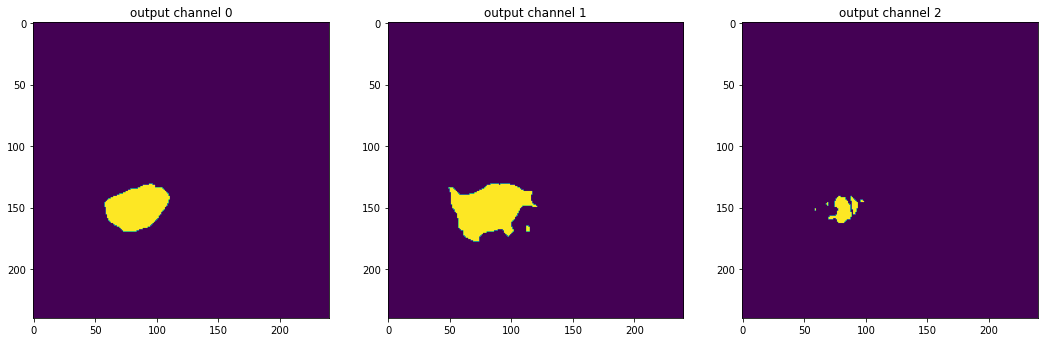
# visualize the 3 channels model output corresponding to this image
plt.figure("output", (18, 6))
for i in range(3):
plt.subplot(1, 3, i + 1)
plt.title(f"output channel {i}")
plt.imshow(val_output[i, :, :, 70].detach().cpu())
plt.show()

元の画像 spacings 上の評価
val_org_transforms = Compose(
    [
        LoadImaged(keys=["image", "label"]),
        EnsureChannelFirstd(keys=["image"]),
        ConvertToMultiChannelBasedOnBratsClassesd(keys="label"),
        Orientationd(keys=["image"], axcodes="RAS"),
        Spacingd(keys=["image"], pixdim=(1.0, 1.0, 1.0), mode="bilinear"),
        NormalizeIntensityd(keys="image", nonzero=True, channel_wise=True),
    ]
)

val_org_ds = DecathlonDataset(
    root_dir=root_dir,
    task="Task01_BrainTumour",
    transform=val_org_transforms,
    section="validation",
    download=False,
    num_workers=4,
    cache_num=0,
)
val_org_loader = DataLoader(val_org_ds, batch_size=1, shuffle=False, num_workers=4)

post_transforms = Compose([
    Invertd(
        keys="pred",
        transform=val_org_transforms,
        orig_keys="image",
        meta_keys="pred_meta_dict",
        orig_meta_keys="image_meta_dict",
        meta_key_postfix="meta_dict",
        nearest_interp=False,
        to_tensor=True,
        device="cpu",
    ),
    Activationsd(keys="pred", sigmoid=True),
    AsDiscreted(keys="pred", threshold=0.5),
])
model.load_state_dict(torch.load(
    os.path.join(root_dir, "best_metric_model.pth")))
model.eval()

with torch.no_grad():
    for val_data in val_org_loader:
        val_inputs = val_data["image"].to(device)
        val_data["pred"] = inference(val_inputs)
        val_data = [post_transforms(i) for i in decollate_batch(val_data)]
        val_outputs, val_labels = from_engine(["pred", "label"])(val_data)
        dice_metric(y_pred=val_outputs, y=val_labels)
        dice_metric_batch(y_pred=val_outputs, y=val_labels)

    metric_org = dice_metric.aggregate().item()
    metric_batch_org = dice_metric_batch.aggregate()

    dice_metric.reset()
    dice_metric_batch.reset()

metric_tc, metric_wt, metric_et = metric_batch_org[0].item(), metric_batch_org[1].item(), metric_batch_org[2].item()

print("Metric on original image spacing: ", metric_org)
print(f"metric_tc: {metric_tc:.4f}")
print(f"metric_wt: {metric_wt:.4f}")
print(f"metric_et: {metric_et:.4f}")
Metric on original image spacing:  0.7912478446960449
metric_tc: 0.8422
metric_wt: 0.9129
metric_et: 0.6187
データディレクトリのクリーンアップ
一時ディレクトリが使用された場合ディレクトリを削除します。
if directory is None:
    shutil.rmtree(root_dir)
以上
MONAI 1.0 : tutorials : モジュール – GAN ワークフロー・エンジン (辞書版)
MONAI 1.0 : tutorials : モジュール – GAN ワークフロー・エンジン (辞書版) (翻訳/解説)
翻訳 : (株)クラスキャット セールスインフォメーション
作成日時 : 11/13/2022 (1.0.1)
* 本ページは、MONAI の以下のドキュメントを翻訳した上で適宜、補足説明したものです:
* サンプルコードの動作確認はしておりますが、必要な場合には適宜、追加改変しています。
* ご自由にリンクを張って頂いてかまいませんが、sales-info@classcat.com までご一報いただけると嬉しいです。
MONAI 1.0 : tutorials : モジュール – GAN ワークフロー・エンジン (辞書版)
このノートブックは GanTrainer、モジュール化された敵対的学習のための MONAI ワークフロー・エンジンを紹介します。MedNIST ハンド CT スキャン・データセットを使用して医用画像再構築ネットワークを訓練します。辞書バージョンです。
MONAI フレームワークは敵対的生成ネットワークを簡単に設計し、訓練して評価するために使用できます。このノートブックは、ハンド CT スキャンの画像を再構築するために単純な GAN モデルを設計して訓練する MONAI コンポーネントを使用する実例を示します。
ネットワーク・アーキテクチャと損失関数の詳細は MONAI Mednist GAN チュートリアル を読んでください。
Step 1: セットアップ
環境のセットアップ
!python -c "import monai" || pip install -q "monai-weekly[ignite, tqdm]"
!python -c "import matplotlib" || pip install -q matplotlib
%matplotlib inline
from monai.utils import set_determinism
from monai.transforms import (
    AddChannelD,
    Compose,
    LoadImageD,
    RandFlipD,
    RandRotateD,
    RandZoomD,
    ScaleIntensityD,
    EnsureTypeD,
)
from monai.networks.nets import Discriminator, Generator
from monai.networks import normal_init
from monai.handlers import CheckpointSaver, MetricLogger, StatsHandler
from monai.engines.utils import GanKeys, default_make_latent
from monai.engines import GanTrainer
from monai.data import CacheDataset, DataLoader
from monai.config import print_config
from monai.apps import download_and_extract
import numpy as np
import torch
import matplotlib.pyplot as plt
import tempfile
import sys
import shutil
import os
import logging
インポートのセットアップ
print_config()
MONAI version: 0.6.0rc1+23.gc6793fd0
Numpy version: 1.20.3
Pytorch version: 1.9.0a0+c3d40fd
MONAI flags: HAS_EXT = True, USE_COMPILED = False
MONAI rev id: c6793fd0f316a448778d0047664aaf8c1895fe1c

Optional dependencies:
Pytorch Ignite version: 0.4.5
Nibabel version: 3.2.1
scikit-image version: 0.15.0
Pillow version: 7.0.0
Tensorboard version: 2.5.0
gdown version: 3.13.0
TorchVision version: 0.10.0a0
ITK version: 5.1.2
tqdm version: 4.53.0
lmdb version: 1.2.1
psutil version: 5.8.0
pandas version: 1.1.4
einops version: 0.3.0

For details about installing the optional dependencies, please visit:
    https://docs.monai.io/en/latest/installation.html#installing-the-recommended-dependencies
データディレクトリのセットアップ
MONAI_DATA_DIRECTORY 環境変数でディレクトリを指定できます。
これは結果をセーブしてダウンロードを再利用することを可能にします。
指定されない場合、一時ディレクトリが使用されます。
directory = os.environ.get("MONAI_DATA_DIRECTORY")
root_dir = tempfile.mkdtemp() if directory is None else directory
print(root_dir)
/workspace/data/medical
データセットをダウンロードする
データセットをダウンロードして展開します。
MedMNIST データセットは TCIA, RSNA Bone Age チャレンジ と NIH Chest X-ray データセット からの様々なセットから集められました。
データセットは Dr. Bradley J. Erickson M.D., Ph.D. (Department of Radiology, Mayo Clinic) のお陰により Creative Commons CC BY-SA 4.0 ライセンス のもとで利用可能になっています。
MedNIST データセットを使用する場合、出典を明示してください、e.g. https://github.com/Project-MONAI/tutorials/blob/master/2d_classification/mednist_tutorial.ipynb。
resource = "https://github.com/Project-MONAI/MONAI-extra-test-data/releases/download/0.8.1/MedNIST.tar.gz"
md5 = "0bc7306e7427e00ad1c5526a6677552d"

compressed_file = os.path.join(root_dir, "MedNIST.tar.gz")
data_dir = os.path.join(root_dir, "MedNIST")
if not os.path.exists(data_dir):
    download_and_extract(resource, compressed_file, root_dir, md5)
hand_dir = os.path.join(data_dir, "Hand")
training_datadict = [
    {"hand": os.path.join(hand_dir, filename)}
    for filename in os.listdir(hand_dir)
]
print(training_datadict[:5])
[{'hand': '/workspace/data/medical/MedNIST/Hand/000317.jpeg'}, {'hand': '/workspace/data/medical/MedNIST/Hand/002344.jpeg'}, {'hand': '/workspace/data/medical/MedNIST/Hand/000816.jpeg'}, {'hand': '/workspace/data/medical/MedNIST/Hand/004046.jpeg'}, {'hand': '/workspace/data/medical/MedNIST/Hand/003316.jpeg'}]
Step 2: MONAI コンポーネントを初期化する
logging.basicConfig(stream=sys.stdout, level=logging.INFO)
set_determinism(0)
device = torch.device("cuda:0")
画像変換チェインを作成する
セーブされたディスク画像を利用可能なテンソルに変換するために処理パイプラインを定義します。
train_transforms = Compose(
    [
        LoadImageD(keys=["hand"]),
        AddChannelD(keys=["hand"]),
        ScaleIntensityD(keys=["hand"]),
        RandRotateD(keys=["hand"], range_x=np.pi /
                    12, prob=0.5, keep_size=True),
        RandFlipD(keys=["hand"], spatial_axis=0, prob=0.5),
        RandZoomD(keys=["hand"], min_zoom=0.9, max_zoom=1.1, prob=0.5),
        EnsureTypeD(keys=["hand"]),
    ]
)
データセットとデータローダを作成する
データを保持して訓練の間にバッチを提示します。
real_dataset = CacheDataset(training_datadict, train_transforms)
100%|██████████| 10000/10000 [00:09<00:00, 1000.72it/s]
batch_size = 300
real_dataloader = DataLoader(
    real_dataset, batch_size=batch_size, shuffle=True, num_workers=10)


def prepare_batch(batchdata, device=None, non_blocking=False):
    return batchdata["hand"].to(device=device, non_blocking=non_blocking)
generator と discriminator を定義する
基本的なコンピュータビジョン GAN ネットワークをライブラリからロードします。
# define networks
disc_net = Discriminator(
    in_shape=(1, 64, 64),
    channels=(8, 16, 32, 64, 1),
    strides=(2, 2, 2, 2, 1),
    num_res_units=1,
    kernel_size=5,
).to(device)

latent_size = 64
gen_net = Generator(
    latent_shape=latent_size,
    start_shape=(latent_size, 8, 8),
    channels=[32, 16, 8, 1],
    strides=[2, 2, 2, 1],
)
gen_net.conv.add_module("activation", torch.nn.Sigmoid())
gen_net = gen_net.to(device)

# initialize both networks
disc_net.apply(normal_init)
gen_net.apply(normal_init)

# define optimizors
learning_rate = 2e-4
betas = (0.5, 0.999)
disc_opt = torch.optim.Adam(disc_net.parameters(), learning_rate, betas=betas)
gen_opt = torch.optim.Adam(gen_net.parameters(), learning_rate, betas=betas)

# define loss functions
disc_loss_criterion = torch.nn.BCELoss()
gen_loss_criterion = torch.nn.BCELoss()
real_label = 1
fake_label = 0


def discriminator_loss(gen_images, real_images):
    real = real_images.new_full((real_images.shape[0], 1), real_label)
    gen = gen_images.new_full((gen_images.shape[0], 1), fake_label)

    realloss = disc_loss_criterion(disc_net(real_images), real)
    genloss = disc_loss_criterion(disc_net(gen_images.detach()), gen)

    return (genloss + realloss) / 2


def generator_loss(gen_images):
    output = disc_net(gen_images)
    cats = output.new_full(output.shape, real_label)
    return gen_loss_criterion(output, cats)
訓練ハンドラを作成する
モデル訓練の間に操作を実行します。
metric_logger = MetricLogger(
    loss_transform=lambda x: {
        GanKeys.GLOSS: x[GanKeys.GLOSS], GanKeys.DLOSS: x[GanKeys.DLOSS]},
    metric_transform=lambda x: x,
)

handlers = [
    StatsHandler(
        name="batch_training_loss",
        output_transform=lambda x: {
            GanKeys.GLOSS: x[GanKeys.GLOSS],
            GanKeys.DLOSS: x[GanKeys.DLOSS],
        },
    ),
    CheckpointSaver(
        save_dir=os.path.join(root_dir, "hand-gan"),
        save_dict={"g_net": gen_net, "d_net": disc_net},
        save_interval=10,
        save_final=True,
        epoch_level=True,
    ),
    metric_logger,
]
GanTrainer を作成する
敵対的学習のための MONAI ワークフロー・エンジン。GanTrainer によってコンポーネントはここで集められます。
Goodfellow et al. 2014 https://arxiv.org/abs/1406.2661 に基づいた訓練ループを使用します。
- ランダムな潜在コードから m 個の fakes を生成します。
- これらの fakes と現在のバッチ reals で D を更新します、d_train_steps 回反復されます。
- 新しいランダムな潜在コードから m fakes を生成します。
- discriminator フィードバックを使用してこれらの fakes で generator を更新します。
disc_train_steps = 5
max_epochs = 50

trainer = GanTrainer(
    device,
    max_epochs,
    real_dataloader,
    gen_net,
    gen_opt,
    generator_loss,
    disc_net,
    disc_opt,
    discriminator_loss,
    d_prepare_batch=prepare_batch,
    d_train_steps=disc_train_steps,
    g_update_latents=True,
    latent_shape=latent_size,
    key_train_metric=None,
    train_handlers=handlers,
)
Step 3: 訓練の開始
trainer.run()
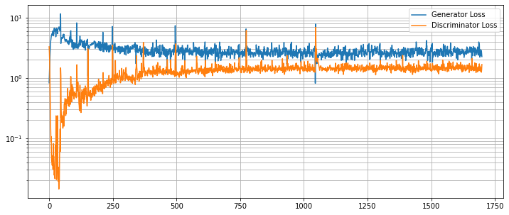
結果を評価する
G と D の損失カーブを崩れていないか調べます。
g_loss = [loss[1][GanKeys.GLOSS] for loss in metric_logger.loss]
d_loss = [loss[1][GanKeys.DLOSS] for loss in metric_logger.loss]
plt.figure(figsize=(12, 5))
plt.semilogy(g_loss, label="Generator Loss")
plt.semilogy(d_loss, label="Discriminator Loss")
plt.grid(True, "both", "both")
plt.legend()
plt.show()
画像再構築を見る
ランダムな潜在コードで訓練された generator の出力を見ます。
test_img_count = 10
test_latents = default_make_latent(test_img_count, latent_size).to(device)
fakes = gen_net(test_latents)

fig, axs = plt.subplots(2, (test_img_count // 2), figsize=(20, 8))
axs = axs.flatten()
for i, ax in enumerate(axs):
    ax.axis("off")
    ax.imshow(fakes[i, 0].cpu().data.numpy(), cmap="gray")
データディレクトリのクリーンアップ
一時ディレクトリが作成された場合にはディレクトリを削除します。
if directory is None:
    shutil.rmtree(root_dir)
以上
MONAI 1.0 : tutorials : モジュール – 2D 画像変換デモ
MONAI 1.0 : tutorials : モジュール – 2D 画像変換デモ (翻訳/解説)
翻訳 : (株)クラスキャット セールスインフォメーション
作成日時 : 11/11/2022 (1.0.1)
* 本ページは、MONAI の以下のドキュメントを翻訳した上で適宜、補足説明したものです:
* サンプルコードの動作確認はしておりますが、必要な場合には適宜、追加改変しています。
* ご自由にリンクを張って頂いてかまいませんが、sales-info@classcat.com までご一報いただけると嬉しいです。
![]()
MONAI 1.0 : tutorials : モジュール – 2D 画像変換デモ
このノートブックは GlaS Contest データセット を使用して組織学 (= histology) の画像の画像変換を実演します。
このデモは MONAI の 2D 変換を適用する方法を示します。主な特徴は :
- ネイティブ PyTorch で実装されたランダムな elastic 変換
- pythonic な方法で設計されて実装された使いやすいインターフェイス
詳細は MONAI の wiki ページで調べてください : https://github.com/Project-MONAI/MONAI/wiki
環境のセットアップ
!python -c "import monai" || pip install -q "monai-weekly[pillow,tqdm]"
!python -c "import matplotlib" || pip install -q matplotlib
%matplotlib inline
from monai.transforms import Affine, Rand2DElastic
from monai.config import print_config
from monai.apps import download_and_extract
import torch
import PIL
import numpy as np
import matplotlib.pyplot as plt
import tempfile
import shutil
import os
インポートのセットアップ
# Copyright 2020 MONAI Consortium
# Licensed under the Apache License, Version 2.0 (the "License");
# you may not use this file except in compliance with the License.
# You may obtain a copy of the License at
#     http://www.apache.org/licenses/LICENSE-2.0
# Unless required by applicable law or agreed to in writing, software
# distributed under the License is distributed on an "AS IS" BASIS,
# WITHOUT WARRANTIES OR CONDITIONS OF ANY KIND, either express or implied.
# See the License for the specific language governing permissions and
# limitations under the License.


print_config()
MONAI version: 0.6.0+135.g3cb355bb
Numpy version: 1.21.2
Pytorch version: 1.9.0
MONAI flags: HAS_EXT = False, USE_COMPILED = False
MONAI rev id: 3cb355bb4e50702a17854cea1b817076c021c1b5

Optional dependencies:
Pytorch Ignite version: 0.4.5
Nibabel version: 3.2.1
scikit-image version: 0.18.3
Pillow version: 8.3.2
Tensorboard version: 2.6.0
gdown version: 3.13.0
TorchVision version: 0.10.0
tqdm version: 4.62.2
lmdb version: 1.2.1
psutil version: 5.8.0
pandas version: 1.3.3
einops version: 0.3.2

For details about installing the optional dependencies, please visit:
    https://docs.monai.io/en/latest/installation.html#installing-the-recommended-dependencies
データディレクトリのセットアップ
MONAI_DATA_DIRECTORY 環境変数でディレクトリを指定できます。
これは結果をセーブしてダウンロードを再利用することを可能にします。
指定されない場合、一時ディレクトリが使用されます。
directory = os.environ.get("MONAI_DATA_DIRECTORY")
root_dir = tempfile.mkdtemp() if directory is None else directory
print(root_dir)
/var/folders/6f/fdkl7m0x7sz3nj_t7p3ccgz00000gp/T/tmpo87g5vor
データセットのダウンロード
データセットをダウンロードして解凍します。データセットは https://warwick.ac.uk/fac/sci/dcs/research/tia/glascontest/ に由来します。
このコンペで使用されたデータセットは研究目的のみで提供されます。商用利用は許容されません。
K. Sirinukunwattana, J. P. W. Pluim, H. Chen, X Qi, P. Heng, Y. Guo, L. Wang, B. J. Matuszewski, E. Bruni, U. Sanchez, A. Böhm, O. Ronneberger, B. Ben Cheikh, D. Racoceanu, P. Kainz, M. Pfeiffer, M. Urschler, D. R. J. Snead, N. M. Rajpoot, “Gland Segmentation in Colon Histology Images: The GlaS Challenge Contest” http://arxiv.org/abs/1603.00275
K. Sirinukunwattana, D.R.J. Snead, N.M. Rajpoot, “A Stochastic Polygons Model for Glandular Structures in Colon Histology Images,” in IEEE Transactions on Medical Imaging, 2015 doi: 10.1109/TMI.2015.2433900
resource = "https://warwick.ac.uk/fac/sci/dcs/research/tia/" \
    + "glascontest/download/warwick_qu_dataset_released_2016_07_08.zip"
md5 = None

compressed_file = os.path.join(
    root_dir, "warwick_qu_dataset_released_2016_07_08.zip")
data_dir = os.path.join(root_dir, "Warwick QU Dataset (Released 2016_07_08)")
if not os.path.exists(data_dir):
    download_and_extract(resource, compressed_file, root_dir, md5)
warwick_qu_dataset_released_2016_07_08.zip: 173MB [00:20, 8.95MB/s]
Downloaded: /var/folders/6f/fdkl7m0x7sz3nj_t7p3ccgz00000gp/T/tmpo87g5vor/warwick_qu_dataset_released_2016_07_08.zip
Expected md5 is None, skip md5 check for file /var/folders/6f/fdkl7m0x7sz3nj_t7p3ccgz00000gp/T/tmpo87g5vor/warwick_qu_dataset_released_2016_07_08.zip.
Writing into directory: /var/folders/6f/fdkl7m0x7sz3nj_t7p3ccgz00000gp/T/tmpo87g5vor.
device = "cpu" if not torch.cuda.is_available() else "cuda:0"
img_name = os.path.join(data_dir, "train_22.bmp")
seg_name = os.path.join(data_dir, "train_22_anno.bmp")
im = np.array(PIL.Image.open(img_name))
seg = np.array(PIL.Image.open(seg_name))
plt.figure("check", (12, 6))
plt.subplot(1, 2, 1)
plt.title("image")
plt.imshow(im)
plt.subplot(1, 2, 2)
plt.title("label")
plt.imshow(seg)
plt.show()
print(im.shape, seg.shape)
![]()
(522, 775, 3) (522, 775)
アフィン変換
# MONAI transforms always take channel-first data: [channel x H x W]
im_data = np.moveaxis(im, -1, 0)  # make them channel first
seg_data = np.expand_dims(seg, 0)  # make a channel for the segmentation

# create an Affine transform
affine = Affine(
    rotate_params=np.pi / 4,
    scale_params=(1.2, 1.2),
    translate_params=(200, 40),
    padding_mode="zeros",
    device=device,
)
# convert both image and segmentation using different interpolation mode
new_img, _ = affine(im_data, (300, 400), mode="bilinear")
new_seg, _ = affine(seg_data, (300, 400), mode="nearest")
print(new_img.shape, new_seg.shape)
(3, 300, 400) (1, 300, 400)
plt.figure("check", (12, 6))
plt.subplot(1, 2, 1)
plt.title("image")
plt.imshow(np.moveaxis(new_img.astype(int), 0, -1))
plt.subplot(1, 2, 2)
plt.title("label")
plt.imshow(new_seg[0].astype(int))
plt.show()
![]()
Elastic 変形 (= deformation)
# create an elsatic deformation transform
deform = Rand2DElastic(
    prob=1.0,
    spacing=(30, 30),
    magnitude_range=(5, 6),
    rotate_range=(np.pi / 4,),
    scale_range=(0.2, 0.2),
    translate_range=(100, 100),
    padding_mode="zeros",
    device=device,
)
# transform both image and segmentation using different interpolation mode
deform.set_random_state(seed=123)
new_img = deform(im_data, (224, 224), mode="bilinear")
deform.set_random_state(seed=123)
new_seg = deform(seg_data, (224, 224), mode="nearest")
print(new_img.shape, new_seg.shape)
(3, 224, 224) (1, 224, 224)
plt.figure("check", (12, 6))
plt.subplot(1, 2, 1)
plt.title("image")
plt.imshow(np.moveaxis(new_img.astype(int), 0, -1))
plt.subplot(1, 2, 2)
plt.title("label")
plt.imshow(new_seg[0].astype(int))
plt.show()
![]()
データディレクトリのクリーンアップ
一時ディレクトリが使用された場合ディレクトリを削除します。
if directory is None:
    shutil.rmtree(root_dir)
以上
MONAI 1.0 : tutorials : モジュール – MedNIST で GAN
MONAI 1.0 : tutorials : モジュール – MedNIST で GAN (翻訳/解説)
翻訳 : (株)クラスキャット セールスインフォメーション
作成日時 : 11/08/2021 (1.0.1)
* 本ページは、MONAI の以下のドキュメントを翻訳した上で適宜、補足説明したものです:
* サンプルコードの動作確認はしておりますが、必要な場合には適宜、追加改変しています。
* ご自由にリンクを張って頂いてかまいませんが、sales-info@classcat.com までご一報いただけると嬉しいです。
- 人工知能研究開発支援
- 人工知能研修サービス(経営者層向けオンサイト研修)
- テクニカルコンサルティングサービス
- 実証実験(プロトタイプ構築)
- アプリケーションへの実装
- 人工知能研修サービス
- PoC(概念実証)を失敗させないための支援
- お住まいの地域に関係なく Web ブラウザからご参加頂けます。事前登録 が必要ですのでご注意ください。
◆ お問合せ : 本件に関するお問い合わせ先は下記までお願いいたします。
- 株式会社クラスキャット セールス・マーケティング本部 セールス・インフォメーション
- sales-info@classcat.com ; Web: www.classcat.com ; ClassCatJP
MONAI 1.0 : tutorials : モジュール – MedNIST で GAN
このノートブックはランダムな入力テンソルから画像を生成するネットワークを訓練するための MONAI の使用方法を例示します。個別の Generator と Discriminator ネットワークに対処する単純な GAN が採用されます。
これは以下のステップを進みます :
- 遠隔ソースからデータをロードする
- このデータからのデータセットと変換を構築する
- ネットワークを定義する
- 訓練と評価
環境セットアップ
!python -c "import monai" || pip install -q monai-weekly
!python -c "import matplotlib" || pip install -q matplotlib
%matplotlib inline
from monai.utils import progress_bar, set_determinism
from monai.transforms import (
    AddChannel,
    Compose,
    RandFlip,
    RandRotate,
    RandZoom,
    ScaleIntensity,
    EnsureType,
    Transform,
)
from monai.networks.nets import Discriminator, Generator
from monai.networks import normal_init
from monai.data import CacheDataset
from monai.config import print_config
from monai.apps import download_and_extract
import numpy as np
import torch
import matplotlib.pyplot as plt
import os
import tempfile
インポートのセットアップ
# Copyright 2020 MONAI Consortium
# Licensed under the Apache License, Version 2.0 (the "License");
# you may not use this file except in compliance with the License.
# You may obtain a copy of the License at
#     http://www.apache.org/licenses/LICENSE-2.0
# Unless required by applicable law or agreed to in writing, software
# distributed under the License is distributed on an "AS IS" BASIS,
# WITHOUT WARRANTIES OR CONDITIONS OF ANY KIND, either express or implied.
# See the License for the specific language governing permissions and
# limitations under the License.


print_config()
MONAI version: 0.6.0rc1+23.gc6793fd0
Numpy version: 1.20.3
Pytorch version: 1.9.0a0+c3d40fd
MONAI flags: HAS_EXT = True, USE_COMPILED = False
MONAI rev id: c6793fd0f316a448778d0047664aaf8c1895fe1c

Optional dependencies:
Pytorch Ignite version: 0.4.5
Nibabel version: 3.2.1
scikit-image version: 0.15.0
Pillow version: 7.0.0
Tensorboard version: 2.5.0
gdown version: 3.13.0
TorchVision version: 0.10.0a0
ITK version: 5.1.2
tqdm version: 4.53.0
lmdb version: 1.2.1
psutil version: 5.8.0
pandas version: 1.1.4
einops version: 0.3.0

For details about installing the optional dependencies, please visit:
    https://docs.monai.io/en/latest/installation.html#installing-the-recommended-dependencies
再現性のための決定論的訓練
set_determinism(seed=0)
訓練変数の定義
disc_train_interval = 1
disc_train_steps = 5
batch_size = 300
latent_size = 64
max_epochs = 50
real_label = 1
gen_label = 0
learning_rate = 2e-4
betas = (0.5, 0.999)
データディレクトリのセットアップ
MONAI_DATA_DIRECTORY 環境変数でディレクトリを指定できます。
これは結果をセーブしてダウンロードを再利用することを可能にします。
指定されない場合、一時ディレクトリが使用されます。
directory = os.environ.get("MONAI_DATA_DIRECTORY")
root_dir = tempfile.mkdtemp() if directory is None else directory
print(root_dir)
/workspace/data/medical
データセットをダウンロードする
MedMNIST データセットは TCIA, RSNA Bone Age チャレンジ と NIH Chest X-ray データセット からの様々なセットから集められました。
データセットは Dr. Bradley J. Erickson M.D., Ph.D. (Department of Radiology, Mayo Clinic) のお陰により Creative Commons CC BY-SA 4.0 ライセンス のもとで利用可能になっています。
MedNIST データセットを使用する場合、出典を明示してください、e.g. https://github.com/Project-MONAI/tutorials/blob/master/2d_classification/mednist_tutorial.ipynb。
ここではファイルシステムを使用することなく tar ファイルからダウンロードして読む方法を示すためと、ハンド X-rays の画像だけを望むために、遠隔ソースからデータをロードする方法は異なります。これは分類サンプルではないのでカテゴリーデータは必要ありませんので、tarball をダウンロードし、標準ライブラリを使用してそれをオープンし、そしてハンドのためのファイル名の総てを recall します :
resource = "https://github.com/Project-MONAI/MONAI-extra-test-data/releases/download/0.8.1/MedNIST.tar.gz"
md5 = "0bc7306e7427e00ad1c5526a6677552d"

compressed_file = os.path.join(root_dir, "MedNIST.tar.gz")
data_dir = os.path.join(root_dir, "MedNIST")
if not os.path.exists(data_dir):
    download_and_extract(resource, compressed_file, root_dir, md5)

hands = [
    os.path.join(data_dir, "Hand", x)
    for x in os.listdir(os.path.join(data_dir, "Hand"))
]
tarfile から実際の画像データをロードするため、Matplotlib を使用してこれを行なう変換タイプを定義します。これはデータを準備するために他の変換とともに使用され、ランダム化された増強変換が続きます。ここでは tarball からの準備された画像の総てをキャッシュするために CacheDataset クラスが使用されますので、ランダム化された回転、反転とズーム操作により増強されることになる準備された画像の総てをメモリに持ちます :
class LoadTarJpeg(Transform):
    def __call__(self, data):
        return plt.imread(data)


train_transforms = Compose(
    [
        LoadTarJpeg(),
        AddChannel(),
        ScaleIntensity(),
        RandRotate(range_x=np.pi / 12, prob=0.5, keep_size=True),
        RandFlip(spatial_axis=0, prob=0.5),
        RandZoom(min_zoom=0.9, max_zoom=1.1, prob=0.5),
        EnsureType(),
    ]
)

train_ds = CacheDataset(hands, train_transforms)
train_loader = torch.utils.data.DataLoader(
    train_ds, batch_size=batch_size, shuffle=True, num_workers=10
)
100%|██████████| 10000/10000 [00:05<00:00, 1691.00it/s]
今は generator と discriminator ネットワークを定義します。パラメータは tar ファイルからロードされた (1, 64, 64) の画像サイズに合うように注意深く選択されています。discriminator への入力画像は非常に小さい画像を生成するために 4 回ダウンサンプリングされます、これらは平坦化されて完全結合層への入力として渡されます。generator への入力潜在ベクトルは shape (64, 8, 8) の出力を生成するために完全結合層に渡されます、そしてこれはリアル画像と同じ shape である最終的な出力を生成するために 3 回アップサンプリングされます。結果を改善するためにネットワークは正規化スキームで初期化されます :
device = torch.device("cuda:0")
disc_net = Discriminator(
    in_shape=(1, 64, 64),
    channels=(8, 16, 32, 64, 1),
    strides=(2, 2, 2, 2, 1),
    num_res_units=1,
    kernel_size=5,
).to(device)


gen_net = Generator(
    latent_shape=latent_size, start_shape=(64, 8, 8),
    channels=[32, 16, 8, 1], strides=[2, 2, 2, 1],
)

# initialize both networks
disc_net.apply(normal_init)
gen_net.apply(normal_init)

# input images are scaled to [0,1] so enforce the same of generated outputs
gen_net.conv.add_module("activation", torch.nn.Sigmoid())
gen_net = gen_net.to(device)
今は generator と discriminator のための損失計算プロセスをラップするヘルパー関数とともに使用する損失関数を定義します。optimizer もまた定義します :
disc_loss = torch.nn.BCELoss()
gen_loss = torch.nn.BCELoss()

disc_opt = torch.optim.Adam(disc_net.parameters(), learning_rate, betas=betas)
gen_opt = torch.optim.Adam(gen_net.parameters(), learning_rate, betas=betas)


def discriminator_loss(gen_images, real_images):
    """
    The discriminator loss if calculated by comparing its
    prediction for real and generated images.

    """
    real = real_images.new_full((real_images.shape[0], 1), real_label)
    gen = gen_images.new_full((gen_images.shape[0], 1), gen_label)

    realloss = disc_loss(disc_net(real_images), real)
    genloss = disc_loss(disc_net(gen_images.detach()), gen)

    return (realloss + genloss) / 2


def generator_loss(input):
    """
    The generator loss is calculated by determining how well
    the discriminator was fooled by the generated images.

    """
    output = disc_net(input)
    cats = output.new_full(output.shape, real_label)
    return gen_loss(output, cats)
今は幾つかのエポックの間データセットに渡り反復することにより訓練します。各バッチのための generator 訓練ステージの後、discriminator は同じリアルと生成画像上で幾つかのステップの間訓練されます。
epoch_loss_values = [(0, 0)]
gen_step_loss = []
disc_step_loss = []
step = 0

for epoch in range(max_epochs):
    gen_net.train()
    disc_net.train()
    epoch_loss = 0

    for i, batch_data in enumerate(train_loader):
        progress_bar(
            i, len(
                train_loader),
            f"epoch {epoch + 1}, avg loss: {epoch_loss_values[-1][1]:.4f}",
        )
        real_images = batch_data.to(device)
        latent = torch.randn(real_images.shape[0], latent_size).to(device)

        gen_opt.zero_grad()
        gen_images = gen_net(latent)
        loss = generator_loss(gen_images)
        loss.backward()
        gen_opt.step()
        epoch_loss += loss.item()

        gen_step_loss.append((step, loss.item()))

        if step % disc_train_interval == 0:
            disc_total_loss = 0

            for _ in range(disc_train_steps):
                disc_opt.zero_grad()
                dloss = discriminator_loss(gen_images, real_images)
                dloss.backward()
                disc_opt.step()
                disc_total_loss += dloss.item()

            disc_step_loss.append((step, disc_total_loss / disc_train_steps))

        step += 1

    epoch_loss /= step
    epoch_loss_values.append((step, epoch_loss))
33/34 epoch 50, avg loss: 0.0563 [============================= ]
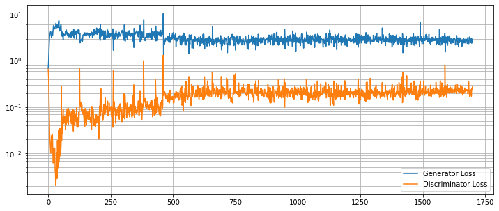
generator と discriminator のための個別の損失値は一緒にグラフ化できます。これらは、discriminator を騙す generator の能力がリアルとフェイク画像の間を正確に識別するネットワークの能力と均衡するにつれて、均衡に達するはずです。
plt.figure(figsize=(12, 5))
plt.semilogy(*zip(*gen_step_loss), label="Generator Loss")
plt.semilogy(*zip(*disc_step_loss), label="Discriminator Loss")
plt.grid(True, "both", "both")
plt.legend()
最後に幾つかランダムに生成された画像を示します。望ましくは期待されるように殆どの画像が 4 本の指と親指を持つことです (polydactyl (= 多指の) サンプルがデータセットに多くは存在していないと仮定して)。このデモ目的のノートブックは長くはネットワークを訓練しません、デフォルトの 50 エポックを越えた訓練は結果を改善するはずです。
test_size = 10
test_latent = torch.randn(test_size, latent_size).to(device)

test_images = gen_net(test_latent)

fig, axs = plt.subplots(1, test_size, figsize=(20, 4))

for i, ax in enumerate(axs):
    ax.axis("off")
    ax.imshow(test_images[i, 0].cpu().data.numpy(), cmap="gray")

以上
MONAI 1.0 : tutorials : 2D レジストレーション – 2D XRay レジストレーション・デモ
MONAI 1.0 : tutorials : 2D レジストレーション – 2D XRay レジストレーション・デモ (翻訳/解説)
翻訳 : (株)クラスキャット セールスインフォメーション
作成日時 : 11/08/2021 (1.0.1)
* 本ページは、MONAI の以下のドキュメントを翻訳した上で適宜、補足説明したものです:
* サンプルコードの動作確認はしておりますが、必要な場合には適宜、追加改変しています。
* ご自由にリンクを張って頂いてかまいませんが、sales-info@classcat.com までご一報いただけると嬉しいです。
- 人工知能研究開発支援
- 人工知能研修サービス(経営者層向けオンサイト研修)
- テクニカルコンサルティングサービス
- 実証実験(プロトタイプ構築)
- アプリケーションへの実装
- 人工知能研修サービス
- PoC(概念実証)を失敗させないための支援
- お住まいの地域に関係なく Web ブラウザからご参加頂けます。事前登録 が必要ですのでご注意ください。
◆ お問合せ : 本件に関するお問い合わせ先は下記までお願いいたします。
- 株式会社クラスキャット セールス・マーケティング本部 セールス・インフォメーション
- sales-info@classcat.com ; Web: www.classcat.com ; ClassCatJP
MONAI 1.0 : tutorials : 2D レジストレーション – 2D XRay レジストレーション・デモ
このノートブックは学習ベースの 64 x 64 X-Ray ハンドのアフィン・レジストレーションの素早いデモを示します。
このデモは MONAI のレジストレーション機能の使用方法を示す toy サンプルです。
このデモは主として以下を使用します :
- アフィン変換パラメータを予測するためにアフィンヘッドを持つ UNet ライクなレジストレーション・ネットワーク ;
- moving 画像を変換するための、MONAI C++/CUDA として実装された、warp 関数。
環境のセットアップ
BUILD_MONAI=1 フラグで “pip install” すると、MONA レポジトリから最新のソースコードを取得し、MONAI の C++/CUDA 拡張を構築して、パッケージをインストールします。
env BUILD_MONAI=1 の設定は、関連する Python モジュールを呼び出すとき MONAI は Pytorch/Python ネイティブ実装の代わりにそれらの拡張を優先することを示します。
(コンパイルは数分から 10+ 分かかる場合があります。)
%env BUILD_MONAI=1
!python -c "import monai" || pip install -q git+https://github.com/Project-MONAI/MONAI#egg=monai[all]
インポートのセットアップ
from monai.utils import set_determinism, first
from monai.transforms import (
    EnsureChannelFirstD,
    Compose,
    LoadImageD,
    RandRotateD,
    RandZoomD,
    ScaleIntensityRanged,
)
from monai.data import DataLoader, Dataset, CacheDataset
from monai.config import print_config, USE_COMPILED
from monai.networks.nets import GlobalNet
from monai.networks.blocks import Warp
from monai.apps import MedNISTDataset

import numpy as np
import torch
from torch.nn import MSELoss
import matplotlib.pyplot as plt
import os
import tempfile


print_config()
set_determinism(42)
MONAI version: 0.5.0+7.g9f4da6a
Numpy version: 1.19.5
Pytorch version: 1.8.1+cu101
MONAI flags: HAS_EXT = True, USE_COMPILED = True
MONAI rev id: 9f4da6acded249bba24c85eaee4ece256ed45815

Optional dependencies:
Pytorch Ignite version: 0.4.4
Nibabel version: 3.0.2
scikit-image version: 0.16.2
Pillow version: 7.1.2
Tensorboard version: 2.4.1
gdown version: 3.6.4
TorchVision version: 0.9.1+cu101
ITK version: 5.1.2
tqdm version: 4.60.0
lmdb version: 0.99
psutil version: 5.4.8

For details about installing the optional dependencies, please visit:
    https://docs.monai.io/en/latest/installation.html#installing-the-recommended-dependencies
データディレクトリのセットアップ
MONAI_DATA_DIRECTORY 環境変数でディレクトリを指定できます。
これは結果をセーブしてダウンロードを再利用することを可能にします。
指定されない場合、一時ディレクトリが使用されます。
directory = os.environ.get("MONAI_DATA_DIRECTORY")
root_dir = tempfile.mkdtemp() if directory is None else directory
print(root_dir)
ペア単位の訓練入力の構築
実際のデータファイルをダウンロードして unzip するために MedNISTDataset オブジェクトを使用します。そして hand クラスを選択し、ロードされたデータ辞書を “fixed_hand” と “moving_hand” に変換します、これらは合成訓練ペアを作成するために別々に前処理されます。
train_data = MedNISTDataset(root_dir=root_dir, section="training", download=True, transform=None)
training_datadict = [
    {"fixed_hand": item["image"], "moving_hand": item["image"]}
    for item in train_data.data if item["label"] == 4  # label 4 is for xray hands
]
print("\n first training items: ", training_datadict[:3])
MedNIST.tar.gz: 59.0MB [00:07, 8.83MB/s]
downloaded file: ./MedNIST.tar.gz.
Verified 'MedNIST.tar.gz', md5: 0bc7306e7427e00ad1c5526a6677552d.
Verified 'MedNIST.tar.gz', md5: 0bc7306e7427e00ad1c5526a6677552d.
Loading dataset: 100%|██████████| 47164/47164 [00:00<00:00, 145309.19it/s]
 first training items:  [{'fixed_hand': './MedNIST/Hand/003696.jpeg', 'moving_hand': './MedNIST/Hand/003696.jpeg'}, {'fixed_hand': './MedNIST/Hand/001404.jpeg', 'moving_hand': './MedNIST/Hand/001404.jpeg'}, {'fixed_hand': './MedNIST/Hand/008882.jpeg', 'moving_hand': './MedNIST/Hand/008882.jpeg'}]
train_transforms = Compose(
    [
        LoadImageD(keys=["fixed_hand", "moving_hand"]),
        EnsureChannelFirstD(keys=["fixed_hand", "moving_hand"]),
        ScaleIntensityRanged(keys=["fixed_hand", "moving_hand"],
                             a_min=0., a_max=255., b_min=0.0, b_max=1.0, clip=True,),
        RandRotateD(keys=["moving_hand"], range_x=np.pi/4, prob=1.0, keep_size=True, mode="bicubic"),
        RandZoomD(keys=["moving_hand"], min_zoom=0.9, max_zoom=1.1, prob=1.0, mode="bicubic", align_corners=False),
    ]
)
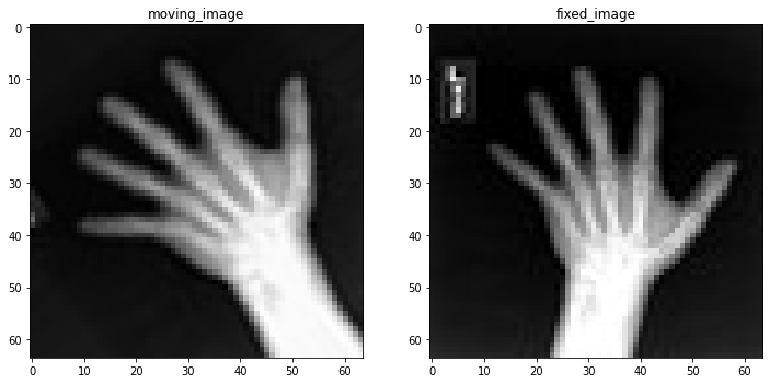
訓練ペアの可視化
check_ds = Dataset(data=training_datadict, transform=train_transforms)
check_loader = DataLoader(check_ds, batch_size=1, shuffle=True)
check_data = first(check_loader)
fixed_image = check_data["fixed_hand"][0][0]
moving_image = check_data["moving_hand"][0][0]

print(f"moving_image shape: {moving_image.shape}")
print(f"fixed_image shape: {fixed_image.shape}")

plt.figure("check", (12, 6))
plt.subplot(1, 2, 1)
plt.title("moving_image")
plt.imshow(moving_image, cmap="gray")
plt.subplot(1, 2, 2)
plt.title("fixed_image")
plt.imshow(fixed_image, cmap="gray")

plt.show()
moving_image shape: torch.Size([64, 64])
fixed_image shape: torch.Size([64, 64])
訓練パイプラインの作成
訓練ペアを capture して訓練プロセスを高速化するために CacheDataset を使用します。この訓練データは GlobalNet に供給されます、これは 画像レベルのアフィン変換パラメータを予測します。Warp 層は初期化されて訓練と推論の両方のために使用されます。
train_ds = CacheDataset(data=training_datadict[:1000], transform=train_transforms,
                        cache_rate=1.0, num_workers=4)
train_loader = DataLoader(train_ds, batch_size=16, shuffle=True, num_workers=2)
Loading dataset: 100%|██████████| 1000/1000 [00:01<00:00, 558.34it/s]
device = torch.device("cuda:0")
model = GlobalNet(
    image_size=(64, 64),
    spatial_dims=2,
    in_channels=2,  # moving and fixed
    num_channel_initial=16,
    depth=3).to(device)
image_loss = MSELoss()
if USE_COMPILED:
    warp_layer = Warp(3, "border").to(device)
else:
    warp_layer = Warp("bilinear", "border").to(device)
optimizer = torch.optim.Adam(model.parameters(), 1e-5)
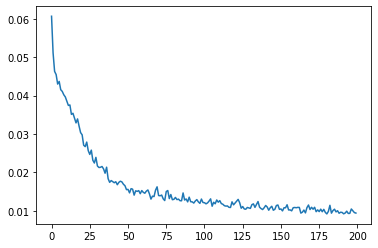
訓練ループ
max_epochs = 200
epoch_loss_values = []

for epoch in range(max_epochs):
    print("-" * 10)
    print(f"epoch {epoch + 1}/{max_epochs}")
    model.train()
    epoch_loss, step = 0, 0
    for batch_data in train_loader:
        step += 1
        optimizer.zero_grad()

        moving = batch_data["moving_hand"].to(device)
        fixed = batch_data["fixed_hand"].to(device)
        ddf = model(torch.cat((moving, fixed), dim=1))
        pred_image = warp_layer(moving, ddf)

        loss = image_loss(pred_image, fixed)
        loss.backward()
        optimizer.step()
        epoch_loss += loss.item()
        # print(f"{step}/{len(train_ds) // train_loader.batch_size}, "
        #       f"train_loss: {loss.item():.4f}")

    epoch_loss /= step
    epoch_loss_values.append(epoch_loss)
    print(f"epoch {epoch + 1} average loss: {epoch_loss:.4f}")
%matplotlib inline
plt.plot(epoch_loss_values)
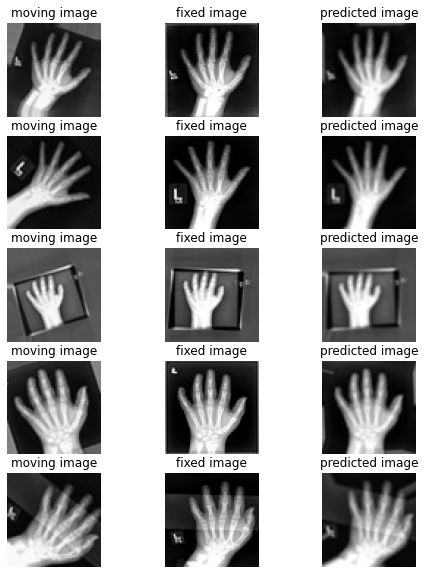
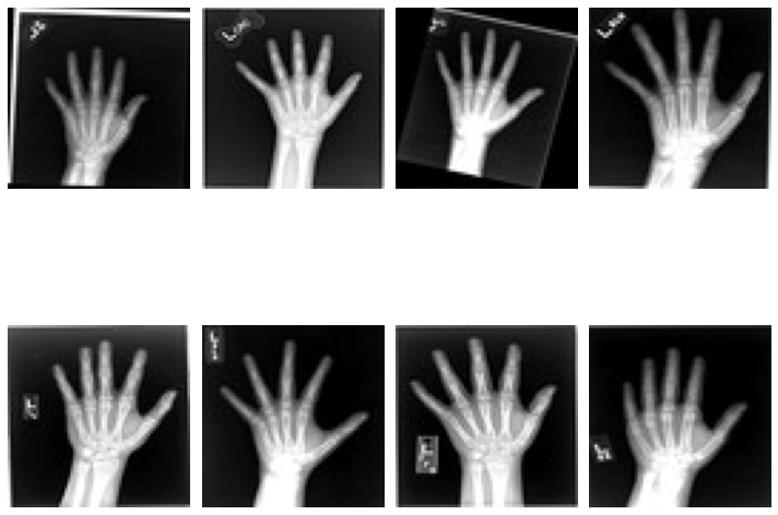
幾つかの検証結果の視覚化
このセクションは moving vs fixed ハンドの未見の (i.e. 前に見てない) ペアのセットを作成して各ペアの間の変換を予測するためにネットワークを使用します。
val_ds = CacheDataset(data=training_datadict[2000:2500], transform=train_transforms,
                      cache_rate=1.0, num_workers=0)
val_loader = DataLoader(val_ds, batch_size=16, num_workers=0)
for batch_data in val_loader:
    moving = batch_data["moving_hand"].to(device)
    fixed = batch_data["fixed_hand"].to(device)
    ddf = model(torch.cat((moving, fixed), dim=1))
    pred_image = warp_layer(moving, ddf)
    break

fixed_image = fixed.detach().cpu().numpy()[:, 0]
moving_image = moving.detach().cpu().numpy()[:, 0]
pred_image = pred_image.detach().cpu().numpy()[:, 0]
Loading dataset: 100%|██████████| 500/500 [00:00<00:00, 803.96it/s]
%matplotlib inline
batch_size = 5
plt.subplots(batch_size, 3, figsize=(8, 10))
for b in range(batch_size):
    # moving image
    plt.subplot(batch_size, 3, b * 3 + 1)
    plt.axis('off')
    plt.title("moving image")
    plt.imshow(moving_image[b], cmap="gray")
    # fixed image
    plt.subplot(batch_size, 3, b * 3 + 2)
    plt.axis('off')
    plt.title("fixed image")
    plt.imshow(fixed_image[b], cmap="gray")
    # warped moving
    plt.subplot(batch_size, 3, b * 3 + 3)
    plt.axis('off')
    plt.title("predicted image")
    plt.imshow(pred_image[b], cmap="gray")
plt.axis('off')
plt.show()
以上
MONAI 1.0 : tutorials : モジュール – MedNIST データセットによる Autoencoder ネットワーク
MONAI 1.0 : tutorials : モジュール – MedNIST データセットによる Autoencoder ネットワーク (翻訳/解説)
翻訳 : (株)クラスキャット セールスインフォメーション
作成日時 : 11/07/2022 (1.0.1)
* 本ページは、MONAI の以下のドキュメントを翻訳した上で適宜、補足説明したものです:
* サンプルコードの動作確認はしておりますが、必要な場合には適宜、追加改変しています。
* ご自由にリンクを張って頂いてかまいませんが、sales-info@classcat.com までご一報いただけると嬉しいです。
- 人工知能研究開発支援
- 人工知能研修サービス(経営者層向けオンサイト研修)
- テクニカルコンサルティングサービス
- 実証実験(プロトタイプ構築)
- アプリケーションへの実装
- 人工知能研修サービス
- PoC(概念実証)を失敗させないための支援
- お住まいの地域に関係なく Web ブラウザからご参加頂けます。事前登録 が必要ですのでご注意ください。
◆ お問合せ : 本件に関するお問い合わせ先は下記までお願いいたします。
- 株式会社クラスキャット セールス・マーケティング本部 セールス・インフォメーション
- sales-info@classcat.com ; Web: www.classcat.com ; ClassCatJP
MONAI 1.0 : tutorials : モジュール – MedNIST データセットによる Autoencoder ネットワーク
このチュートリアルは MONAI の autoencoder クラスを実演するために MedNIST ハンド CT スキャン・データセットを使用します。autoencoder は恒等エンコード/デコードで使用され (i.e. 貴方の入れたものが戻されるべきもの)、そしてぼかしとノイズの除去の使用方法として実演します。
このノートブックは画像のぼかし/ノイズ除去の目的で MONAI で autoencoeder の使用方法を示します。
学習目標
これは以下のステップを進みます :
- 遠隔ソースからデータをロードする
- 画像の辞書を作成するために lambda を使用する
- MONAI の組込み AutoEncoder を使用する
環境のセットアップ
!python -c "import monai" || pip install -q "monai-weekly[pillow, tqdm]"
1. インポートと設定
import logging
import os
import shutil
import sys
import tempfile
import random
import numpy as np
from tqdm import trange
import matplotlib.pyplot as plt
import torch
from skimage.util import random_noise

from monai.apps import download_and_extract
from monai.config import print_config
from monai.data import CacheDataset, DataLoader
from monai.networks.nets import AutoEncoder
from monai.transforms import (
    EnsureChannelFirstD,
    Compose,
    LoadImageD,
    RandFlipD,
    RandRotateD,
    RandZoomD,
    ScaleIntensityD,
    EnsureTypeD,
    Lambda,
)
from monai.utils import set_determinism

print_config()
MONAI version: 0.6.0rc1+23.gc6793fd0
Numpy version: 1.20.3
Pytorch version: 1.9.0a0+c3d40fd
MONAI flags: HAS_EXT = True, USE_COMPILED = False
MONAI rev id: c6793fd0f316a448778d0047664aaf8c1895fe1c

Optional dependencies:
Pytorch Ignite version: 0.4.5
Nibabel version: 3.2.1
scikit-image version: 0.15.0
Pillow version: 8.2.0
Tensorboard version: 2.5.0
gdown version: 3.13.0
TorchVision version: 0.10.0a0
ITK version: 5.1.2
tqdm version: 4.53.0
lmdb version: 1.2.1
psutil version: 5.8.0
pandas version: 1.1.4
einops version: 0.3.0

For details about installing the optional dependencies, please visit:
    https://docs.monai.io/en/latest/installation.html#installing-the-recommended-dependencies
logging.basicConfig(stream=sys.stdout, level=logging.INFO)
set_determinism(0)
device = torch.device("cuda" if torch.cuda.is_available() else "cpu")
# Create small visualisation function
def plot_ims(ims, shape=None, figsize=(10, 10), titles=None):
    shape = (1, len(ims)) if shape is None else shape
    plt.subplots(*shape, figsize=figsize)
    for i, im in enumerate(ims):
        plt.subplot(*shape, i + 1)
        im = plt.imread(im) if isinstance(im, str) else torch.squeeze(im)
        plt.imshow(im, cmap='gray')
        if titles is not None:
            plt.title(titles[i])
        plt.axis('off')
    plt.tight_layout()
    plt.show()
データを取得する
MedMNIST データセットは TCIA, RSNA Bone Age チャレンジ と NIH Chest X-ray データセット からの様々なセットから集められました。
データセットは Dr. Bradley J. Erickson M.D., Ph.D. (Department of Radiology, Mayo Clinic) のお陰により Creative Commons CC BY-SA 4.0 ライセンス のもとで利用可能になっています。
directory = os.environ.get("MONAI_DATA_DIRECTORY")
root_dir = tempfile.mkdtemp() if directory is None else directory
print(root_dir)
/workspace/data/medical
resource = "https://github.com/Project-MONAI/MONAI-extra-test-data/releases/download/0.8.1/MedNIST.tar.gz"
md5 = "0bc7306e7427e00ad1c5526a6677552d"

compressed_file = os.path.join(root_dir, "MedNIST.tar.gz")
data_dir = os.path.join(root_dir, "MedNIST")
if not os.path.exists(data_dir):
    download_and_extract(resource, compressed_file, root_dir, md5)
# scan_type could be AbdomenCT BreastMRI CXR ChestCT Hand HeadCT
scan_type = "Hand"
im_dir = os.path.join(data_dir, scan_type)
all_filenames = [os.path.join(im_dir, filename)
for filename in os.listdir(im_dir)]
random.shuffle(all_filenames)
# Visualise a few of them
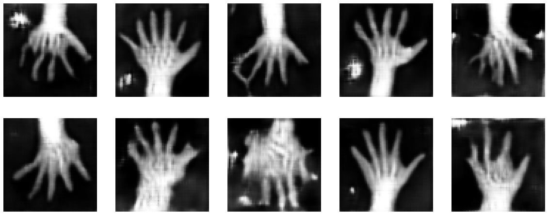
rand_images = np.random.choice(all_filenames, 8, replace=False)
plot_ims(rand_images, shape=(2, 4))
# Split into training and testing
test_frac = 0.2
num_test = int(len(all_filenames) * test_frac)
num_train = len(all_filenames) - num_test
train_datadict = [{"im": fname} for fname in all_filenames[:num_train]]
test_datadict = [{"im": fname} for fname in all_filenames[-num_test:]]
print(f"total number of images: {len(all_filenames)}")
print(f"number of images for training: {len(train_datadict)}")
print(f"number of images for testing: {len(test_datadict)}")
total number of images: 10000
number of images for training: 8000
number of images for testing: 2000
3. 画像変換チェインを作成する
画像のぼやけ/ノイズを除去する autoencoder を訓練するため、劣化画像をエンコーダに渡すことを望みますが、損失関数では、元の劣化していないバージョンとの比較を行ないます。この意味で、エンコードとデコードステップが劣化を除去できたときに、損失関数は最小化されます。
画像の一つのバージョンが劣化していて他方がそうではないという事実以外に、それらが同一であるようにすることを望みます、これは同じ変換から生成される必要があることを意味します。これを行なう最も簡単な方法は辞書変換を使うことです、そこでは最後に、3 つの画像 – オリジナル、ガウスぼかしとノイズのある (画像) を含む辞書を返す lambda 関数を持ちます。
NoiseLambda = Lambda(lambda d: {
    "orig": d["im"],
    "gaus": torch.tensor(
        random_noise(d["im"], mode='gaussian'), dtype=torch.float32),
    "s&p": torch.tensor(random_noise(d["im"], mode='s&p', salt_vs_pepper=0.1)),
})

train_transforms = Compose(
    [
        LoadImageD(keys=["im"]),
        EnsureChannelFirstD(keys=["im"]),
        ScaleIntensityD(keys=["im"]),
        RandRotateD(keys=["im"], range_x=np.pi / 12, prob=0.5, keep_size=True),
        RandFlipD(keys=["im"], spatial_axis=0, prob=0.5),
        RandZoomD(keys=["im"], min_zoom=0.9, max_zoom=1.1, prob=0.5),
        EnsureTypeD(keys=["im"]),
        NoiseLambda,
    ]
)

test_transforms = Compose(
    [
        LoadImageD(keys=["im"]),
        EnsureChannelFirstD(keys=["im"]),
        ScaleIntensityD(keys=["im"]),
        EnsureTypeD(keys=["im"]),
        NoiseLambda,
    ]
)
データセットとデータローダの作成
データを保持して訓練の間にバッチを提示する
batch_size = 300
num_workers = 10

train_ds = CacheDataset(train_datadict, train_transforms,
                        num_workers=num_workers)
train_loader = DataLoader(train_ds, batch_size=batch_size,
                          shuffle=True, num_workers=num_workers)
test_ds = CacheDataset(test_datadict, test_transforms, num_workers=num_workers)
test_loader = DataLoader(test_ds, batch_size=batch_size,
                         shuffle=True, num_workers=num_workers)
100%|██████████| 8000/8000 [00:02<00:00, 2698.01it/s]
100%|██████████| 2000/2000 [00:02<00:00, 904.36it/s]
# Get image original and its degraded versions
def get_single_im(ds):
    loader = torch.utils.data.DataLoader(
        ds, batch_size=1, num_workers=10, shuffle=True)
    itera = iter(loader)
    return next(itera)
data = get_single_im(train_ds)
plot_ims([data['orig'], data['gaus'], data['s&p']],
         titles=['orig', 'Gaussian', 's&p'])
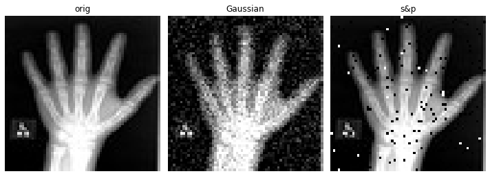
def train(dict_key_for_training, max_epochs=10, learning_rate=1e-3):

    model = AutoEncoder(
        spatial_dims=2,
        in_channels=1,
        out_channels=1,
        channels=(4, 8, 16, 32),
        strides=(2, 2, 2, 2),
    ).to(device)

    # Create loss fn and optimiser
    loss_function = torch.nn.MSELoss()
    optimizer = torch.optim.Adam(model.parameters(), learning_rate)

    epoch_loss_values = []

    t = trange(
        max_epochs,
        desc=f"{dict_key_for_training} -- epoch 0, avg loss: inf", leave=True)
    for epoch in t:
        model.train()
        epoch_loss = 0
        step = 0
        for batch_data in train_loader:
            step += 1
            inputs = batch_data[dict_key_for_training].to(device)
            optimizer.zero_grad()
            outputs = model(inputs)
            loss = loss_function(outputs, batch_data['orig'].to(device))
            loss.backward()
            optimizer.step()
            epoch_loss += loss.item()
        epoch_loss /= step
        epoch_loss_values.append(epoch_loss)
        t.set_description(
            f"{dict_key_for_training} -- epoch {epoch + 1}"
            + f", average loss: {epoch_loss:.4f}")
    return model, epoch_loss_values
max_epochs = 50
training_types = ['orig', 'gaus', 's&p']
models = []
epoch_losses = []
for training_type in training_types:
    model, epoch_loss = train(training_type, max_epochs=max_epochs)
    models.append(model)
    epoch_losses.append(epoch_loss)
orig -- epoch 30, average loss: 0.0110: 60%|██████ | 30/50 [01:41<01:08, 3.40s/it]
plt.figure()
plt.title("Epoch Average Loss")
plt.xlabel("epoch")
for y, label in zip(epoch_losses, training_types):
    x = list(range(1, len(y) + 1))
    line, = plt.plot(x, y)
    line.set_label(label)
plt.legend()
data = get_single_im(test_ds)

recons = []
for model, training_type in zip(models, training_types):
    im = data[training_type]
    recon = model(im.to(device)).detach().cpu()
    recons.append(recon)

plot_ims(
    [data['orig'], data['gaus'], data['s&p']] + recons,
    titles=['orig', 'Gaussian', 'S&P'] +
    ["recon w/\n" + x for x in training_types],
    shape=(2, len(training_types)))
データディレクトリのクリーンアップ
一時ディレクトリが使用された場合ディレクトリを削除します。
if directory is None:
    shutil.rmtree(root_dir)
以上
MONAI 1.0 : チュートリアル
MONAI 1.0 : チュートリアル
翻訳 : (株)クラスキャット セールスインフォメーション
更新日時 : 01/19/2023 (1.1.0)
作成日時 : 11/02/2022 (1.0.1)
- 人工知能研究開発支援
- 人工知能研修サービス(経営者層向けオンサイト研修)
- テクニカルコンサルティングサービス
- 実証実験(プロトタイプ構築)
- アプリケーションへの実装
- 人工知能研修サービス
- PoC(概念実証)を失敗させないための支援
- お住まいの地域に関係なく Web ブラウザからご参加頂けます。事前登録 が必要ですのでご注意ください。
◆ お問合せ : 本件に関するお問い合わせ先は下記までお願いいたします。
- 株式会社クラスキャット セールス・マーケティング本部 セールス・インフォメーション
- sales-info@classcat.com ; Web: www.classcat.com ; ClassCatJP
![]()
MONAI 1.0 : チュートリアル
2D 分類
- MedNIST データセットによる医用画像分類 (2d_classification/mednist_tutorial) (11/02/2022)
3D セグメンテーション
- 脳腫瘍 3D セグメンテーション (brats_segmentation_3d) (01/18/2023)
- 脾臓 3D セグメンテーション (spleen_segmentation_3d) (01/19/2023)
2D レジストレーション
- 2D XRay レジストレーション・デモ (2d_registration/registration_mednist) (11/08/2022)
モジュール
- MedNIST データセットによる Autoencoder ネットワーク (modules/autoencoder_mednist) (11/07/2022)
- MedNIST で GAN (modules/mednist_GAN_tutorial) (11/08/2022)
- GAN ワークフロー・エンジン (辞書版) (mednist_GAN_workflow_dict) (11/13/2022)
- 2D 画像変換デモ (transforms_demo_2d) (11/11/2021)
以上
MONAI 1.0 : tutorials : 2D 分類 – MedNIST データセットによる医用画像分類
MONAI 1.0 : tutorials : 2D 分類 – MedNIST データセットによる医用画像分類 (翻訳/解説)
翻訳 : (株)クラスキャット セールスインフォメーション
作成日時 : 11/01/2022 (1.0.1)
* 本ページは、MONAI の以下のドキュメントを翻訳した上で適宜、補足説明したものです:
* サンプルコードの動作確認はしておりますが、必要な場合には適宜、追加改変しています。
* ご自由にリンクを張って頂いてかまいませんが、sales-info@classcat.com までご一報いただけると嬉しいです。
- 人工知能研究開発支援
- 人工知能研修サービス(経営者層向けオンサイト研修)
- テクニカルコンサルティングサービス
- 実証実験(プロトタイプ構築)
- アプリケーションへの実装
- 人工知能研修サービス
- PoC(概念実証)を失敗させないための支援
- お住まいの地域に関係なく Web ブラウザからご参加頂けます。事前登録 が必要ですのでご注意ください。
◆ お問合せ : 本件に関するお問い合わせ先は下記までお願いいたします。
- 株式会社クラスキャット セールス・マーケティング本部 セールス・インフォメーション
- sales-info@classcat.com ; Web: www.classcat.com ; ClassCatJP
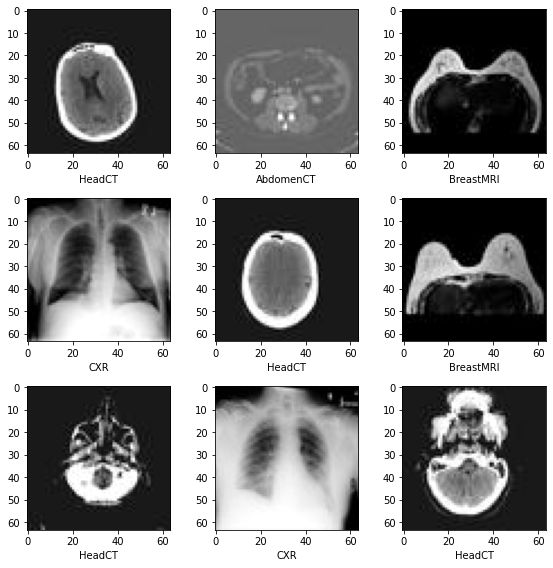
MONAI 1.0 : tutorials : 2D 分類 – MedNIST データセットによる医用画像分類
このノートブックは MONAI 機能を既存の PyTorch プログラムに容易に統合する方法を示します。それは MedNIST データセットに基づいています、これは初心者のためにチュートリアルとして非常に適切です。このチュートリアルはまた MONAI 組込みのオクルージョン感度の機能も利用しています。
このチュートリアルでは、MedNIST データセットに基づく end-to-end な訓練と評価サンプルを紹介します。
以下のステップで進めます :
- 訓練とテスト用のデータセットを作成する。
- データを前処理するために MONAI 変換を利用します。
- 分類のために MONAI から DenseNet を利用します。
- モデルを PyTorch プログラムで訓練します。
- テストデータセット上で評価します。
環境のセットアップ
!python -c "import monai" || pip install -q "monai-weekly[pillow, tqdm]"
!python -c "import matplotlib" || pip install -q matplotlib
%matplotlib inline
インポートのセットアップ
# Copyright 2020 MONAI Consortium
# Licensed under the Apache License, Version 2.0 (the "License");
# you may not use this file except in compliance with the License.
# You may obtain a copy of the License at
#     http://www.apache.org/licenses/LICENSE-2.0
# Unless required by applicable law or agreed to in writing, software
# distributed under the License is distributed on an "AS IS" BASIS,
# WITHOUT WARRANTIES OR CONDITIONS OF ANY KIND, either express or implied.
# See the License for the specific language governing permissions and
# limitations under the License.

import os
import shutil
import tempfile
import matplotlib.pyplot as plt
import PIL
import torch
import numpy as np
from sklearn.metrics import classification_report

from monai.apps import download_and_extract
from monai.config import print_config
from monai.data import decollate_batch, DataLoader
from monai.metrics import ROCAUCMetric
from monai.networks.nets import DenseNet121
from monai.transforms import (
    Activations,
    EnsureChannelFirst,
    AsDiscrete,
    Compose,
    LoadImage,
    RandFlip,
    RandRotate,
    RandZoom,
    ScaleIntensity,
)
from monai.utils import set_determinism

print_config()
MONAI version: 0.9.dev2152
Numpy version: 1.19.5
Pytorch version: 1.10.0+cu111
MONAI flags: HAS_EXT = False, USE_COMPILED = False
MONAI rev id: c5bd8aff8ba461d7b349eb92427d452481a7eb72

Optional dependencies:
Pytorch Ignite version: NOT INSTALLED or UNKNOWN VERSION.
Nibabel version: 3.0.2
scikit-image version: 0.18.3
Pillow version: 7.1.2
Tensorboard version: 2.7.0
gdown version: 3.6.4
TorchVision version: 0.11.1+cu111
tqdm version: 4.62.3
lmdb version: 0.99
psutil version: 5.4.8
pandas version: 1.1.5
einops version: NOT INSTALLED or UNKNOWN VERSION.
transformers version: NOT INSTALLED or UNKNOWN VERSION.
mlflow version: NOT INSTALLED or UNKNOWN VERSION.

For details about installing the optional dependencies, please visit:
    https://docs.monai.io/en/latest/installation.html#installing-the-recommended-dependencies
データディレクトリのセットアップ
MONAI_DATA_DIRECTORY 環境変数でディレクトリを指定できます。これは結果をセーブしてダウンロードを再利用することを可能にします。指定されない場合、一時ディレクトリが使用されます。
directory = os.environ.get("MONAI_DATA_DIRECTORY")
root_dir = tempfile.mkdtemp() if directory is None else directory
print(root_dir)
/workspace/data/medical
データセットをダウンロードする
MedMNIST データセットは TCIA, RSNA Bone Age チャレンジ と NIH Chest X-ray データセット からの様々なセットから集められました。
データセットは Dr. Bradley J. Erickson M.D., Ph.D. (Department of Radiology, Mayo Clinic) のお陰により Creative Commons CC BY-SA 4.0 ライセンス のもとで利用可能になっています。
MedNIST データセットを使用する場合、出典を明示してください。
resource = "https://github.com/Project-MONAI/MONAI-extra-test-data/releases/download/0.8.1/MedNIST.tar.gz"
md5 = "0bc7306e7427e00ad1c5526a6677552d"

compressed_file = os.path.join(root_dir, "MedNIST.tar.gz")
data_dir = os.path.join(root_dir, "MedNIST")
if not os.path.exists(data_dir):
    download_and_extract(resource, compressed_file, root_dir, md5)
再現性のために決定論的訓練を設定する
set_determinism(seed=0)
データセットフォルダから画像ファイル名を読む
まず最初に、データセットファイルを確認して幾つかの統計情報を表示します。
データセットには 6 つのフォルダがあります : Hand, AbdomenCT, CXR, ChestCT, BreastMRI, HeadCT,
これらは分類モデルを訓練するためのラベルとして使用されるべきです。
class_names = sorted(x for x in os.listdir(data_dir)
                     if os.path.isdir(os.path.join(data_dir, x)))
num_class = len(class_names)
image_files = [
    [
        os.path.join(data_dir, class_names[i], x)
        for x in os.listdir(os.path.join(data_dir, class_names[i]))
    ]
    for i in range(num_class)
]
num_each = [len(image_files[i]) for i in range(num_class)]
image_files_list = []
image_class = []
for i in range(num_class):
    image_files_list.extend(image_files[i])
    image_class.extend([i] * num_each[i])
num_total = len(image_class)
image_width, image_height = PIL.Image.open(image_files_list[0]).size

print(f"Total image count: {num_total}")
print(f"Image dimensions: {image_width} x {image_height}")
print(f"Label names: {class_names}")
print(f"Label counts: {num_each}")
Total image count: 58954
Image dimensions: 64 x 64
Label names: ['AbdomenCT', 'BreastMRI', 'CXR', 'ChestCT', 'Hand', 'HeadCT']
Label counts: [10000, 8954, 10000, 10000, 10000, 10000]
データセットから画像をランダムに選択して可視化して確認する
plt.subplots(3, 3, figsize=(8, 8))
for i, k in enumerate(np.random.randint(num_total, size=9)):
    im = PIL.Image.open(image_files_list[k])
    arr = np.array(im)
    plt.subplot(3, 3, i + 1)
    plt.xlabel(class_names[image_class[k]])
    plt.imshow(arr, cmap="gray", vmin=0, vmax=255)
plt.tight_layout()
plt.show()
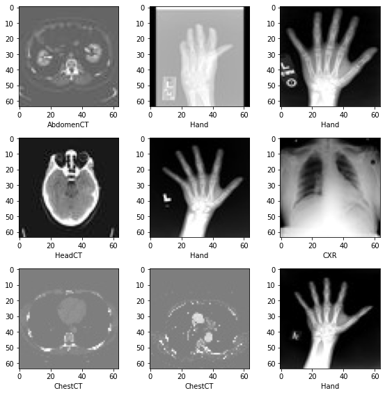
訓練、検証とテストデータのリストを準備する
データセットの 10% を検証用に、そして 10% をテスト用にランダムに選択します。
val_frac = 0.1
test_frac = 0.1
length = len(image_files_list)
indices = np.arange(length)
np.random.shuffle(indices)

test_split = int(test_frac * length)
val_split = int(val_frac * length) + test_split
test_indices = indices[:test_split]
val_indices = indices[test_split:val_split]
train_indices = indices[val_split:]

train_x = [image_files_list[i] for i in train_indices]
train_y = [image_class[i] for i in train_indices]
val_x = [image_files_list[i] for i in val_indices]
val_y = [image_class[i] for i in val_indices]
test_x = [image_files_list[i] for i in test_indices]
test_y = [image_class[i] for i in test_indices]

print(
    f"Training count: {len(train_x)}, Validation count: "
    f"{len(val_x)}, Test count: {len(test_x)}")
Training count: 47156, Validation count: 5913, Test count: 5885
データを前処理するために MONAI 変換、Dataset と Dataloader を定義する
train_transforms = Compose(
    [
        LoadImage(image_only=True),
        EnsureChannelFirst(),
        ScaleIntensity(),
        RandRotate(range_x=np.pi / 12, prob=0.5, keep_size=True),
        RandFlip(spatial_axis=0, prob=0.5),
        RandZoom(min_zoom=0.9, max_zoom=1.1, prob=0.5),
    ]
)

val_transforms = Compose(
    [LoadImage(image_only=True), EnsureChannelFirst(), ScaleIntensity()])

y_pred_trans = Compose([Activations(softmax=True)])
y_trans = Compose([AsDiscrete(to_onehot=num_class)])
class MedNISTDataset(torch.utils.data.Dataset):
    def __init__(self, image_files, labels, transforms):
        self.image_files = image_files
        self.labels = labels
        self.transforms = transforms

    def __len__(self):
        return len(self.image_files)

    def __getitem__(self, index):
        return self.transforms(self.image_files[index]), self.labels[index]


train_ds = MedNISTDataset(train_x, train_y, train_transforms)
train_loader = DataLoader(
    train_ds, batch_size=300, shuffle=True, num_workers=10)

val_ds = MedNISTDataset(val_x, val_y, val_transforms)
val_loader = DataLoader(
    val_ds, batch_size=300, num_workers=10)

test_ds = MedNISTDataset(test_x, test_y, val_transforms)
test_loader = DataLoader(
    test_ds, batch_size=300, num_workers=10)
ネットワークと optimizer を定義する
- バッチ毎にモデルがどのくらい更新されるかについて学習率を設定します。
- 総エポック数を設定します、シャッフルしてランダムな変換を行ないますので、総てのエポックの訓練データは異なります。
そしてこれは get start チュートリアルに過ぎませんので、4 エポックだけ訓練しましょう。
10 エポック訓練すれば、モデルはテストデータセット上で 100% 精度を達成できます。
- MONAI からの DenseNet を使用して GPU デバイスに移します、この DenseNet は 2D と 3D 分類タスクの両方をサポートできます。
- Adam optimizer を使用します。
device = torch.device("cuda" if torch.cuda.is_available() else "cpu")
model = DenseNet121(spatial_dims=2, in_channels=1,
                    out_channels=num_class).to(device)
loss_function = torch.nn.CrossEntropyLoss()
optimizer = torch.optim.Adam(model.parameters(), 1e-5)
max_epochs = 4
val_interval = 1
auc_metric = ROCAUCMetric()
モデル訓練
典型的な PyTorch 訓練を実行します、これはエポック・ループとステップ・ループを実行して、総てのエポック後に検証を行ないます。ベストの検証精度を得た場合、モデル重みをファイルにセーブします。
best_metric = -1
best_metric_epoch = -1
epoch_loss_values = []
metric_values = []

for epoch in range(max_epochs):
    print("-" * 10)
    print(f"epoch {epoch + 1}/{max_epochs}")
    model.train()
    epoch_loss = 0
    step = 0
    for batch_data in train_loader:
        step += 1
        inputs, labels = batch_data[0].to(device), batch_data[1].to(device)
        optimizer.zero_grad()
        outputs = model(inputs)
        loss = loss_function(outputs, labels)
        loss.backward()
        optimizer.step()
        epoch_loss += loss.item()
        print(
            f"{step}/{len(train_ds) // train_loader.batch_size}, "
            f"train_loss: {loss.item():.4f}")
        epoch_len = len(train_ds) // train_loader.batch_size
    epoch_loss /= step
    epoch_loss_values.append(epoch_loss)
    print(f"epoch {epoch + 1} average loss: {epoch_loss:.4f}")

    if (epoch + 1) % val_interval == 0:
        model.eval()
        with torch.no_grad():
            y_pred = torch.tensor([], dtype=torch.float32, device=device)
            y = torch.tensor([], dtype=torch.long, device=device)
            for val_data in val_loader:
                val_images, val_labels = (
                    val_data[0].to(device),
                    val_data[1].to(device),
                )
                y_pred = torch.cat([y_pred, model(val_images)], dim=0)
                y = torch.cat([y, val_labels], dim=0)
            y_onehot = [y_trans(i) for i in decollate_batch(y, detach=False)]
            y_pred_act = [y_pred_trans(i) for i in decollate_batch(y_pred)]
            auc_metric(y_pred_act, y_onehot)
            result = auc_metric.aggregate()
            auc_metric.reset()
            del y_pred_act, y_onehot
            metric_values.append(result)
            acc_value = torch.eq(y_pred.argmax(dim=1), y)
            acc_metric = acc_value.sum().item() / len(acc_value)
            if result > best_metric:
                best_metric = result
                best_metric_epoch = epoch + 1
                torch.save(model.state_dict(), os.path.join(
                    root_dir, "best_metric_model.pth"))
                print("saved new best metric model")
            print(
                f"current epoch: {epoch + 1} current AUC: {result:.4f}"
                f" current accuracy: {acc_metric:.4f}"
                f" best AUC: {best_metric:.4f}"
                f" at epoch: {best_metric_epoch}"
            )

print(
    f"train completed, best_metric: {best_metric:.4f} "
    f"at epoch: {best_metric_epoch}")
----------
epoch 1/4
(...)
epoch 1 average loss: 0.7768
saved new best metric model
current epoch: 1 current AUC: 0.9984 current accuracy: 0.9618 best AUC: 0.9984 at epoch: 1
----------
epoch 2/4
(...)
epoch 2 average loss: 0.1612
saved new best metric model
current epoch: 2 current AUC: 0.9997 current accuracy: 0.9863 best AUC: 0.9997 at epoch: 2
----------
epoch 3/4
(...)
epoch 3 average loss: 0.0743
saved new best metric model
current epoch: 3 current AUC: 0.9999 current accuracy: 0.9924 best AUC: 0.9999 at epoch: 3
----------
epoch 4/4
(...)
epoch 4 average loss: 0.0462
saved new best metric model
current epoch: 4 current AUC: 1.0000 current accuracy: 0.9944 best AUC: 1.0000 at epoch: 4
train completed, best_metric: 1.0000 at epoch: 4
(...)
epoch 9 average loss: 0.0094
saved new best metric model
current epoch: 9 current AUC: 1.0000 current accuracy: 0.9997 best AUC: 1.0000 at epoch: 9
----------
epoch 10/10
(...)
epoch 10 average loss: 0.0080
current epoch: 10 current AUC: 1.0000 current accuracy: 0.9997 best AUC: 1.0000 at epoch: 9
train completed, best_metric: 1.0000 at epoch: 9
損失とメトリックをプロットする
plt.figure("train", (12, 6))
plt.subplot(1, 2, 1)
plt.title("Epoch Average Loss")
x = [i + 1 for i in range(len(epoch_loss_values))]
y = epoch_loss_values
plt.xlabel("epoch")
plt.plot(x, y)
plt.subplot(1, 2, 2)
plt.title("Val AUC")
x = [val_interval * (i + 1) for i in range(len(metric_values))]
y = metric_values
plt.xlabel("epoch")
plt.plot(x, y)
plt.show()
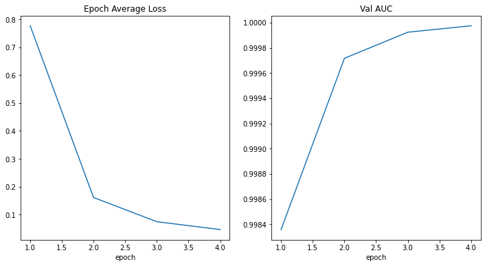
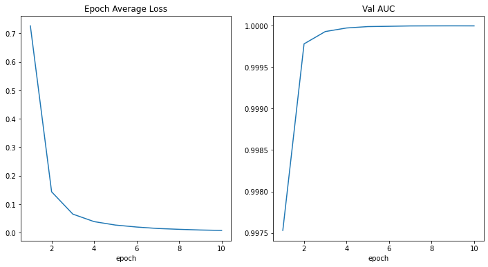
テストデータセット上でモデルを評価する
訓練と検証の後、検証テスト上のベストモデルを既に得ています。
モデルをテストデータセット上でそれが堅牢で over fitting していないかを確認するために評価する必要があります。
分類レポートを生成するためにこれらの予測を使用します。
model.load_state_dict(torch.load(
    os.path.join(root_dir, "best_metric_model.pth")))
model.eval()
y_true = []
y_pred = []
with torch.no_grad():
    for test_data in test_loader:
        test_images, test_labels = (
            test_data[0].to(device),
            test_data[1].to(device),
        )
        pred = model(test_images).argmax(dim=1)
        for i in range(len(pred)):
            y_true.append(test_labels[i].item())
            y_pred.append(pred[i].item())
print(classification_report(
    y_true, y_pred, target_names=class_names, digits=4))
Note: you may need to restart the kernel to use updated packages.
              precision    recall  f1-score   support

   AbdomenCT     0.9816    0.9917    0.9867       969
   BreastMRI     0.9968    0.9831    0.9899       944
         CXR     0.9979    0.9928    0.9954       973
     ChestCT     0.9938    0.9990    0.9964       959
        Hand     0.9934    0.9934    0.9934      1055
      HeadCT     0.9960    0.9990    0.9975       985

    accuracy                         0.9932      5885
   macro avg     0.9932    0.9932    0.9932      5885
weighted avg     0.9932    0.9932    0.9932      5885
              precision    recall  f1-score   support

   AbdomenCT     0.9980    0.9990    0.9985       995
   BreastMRI     0.9989    1.0000    0.9994       880
         CXR     1.0000    0.9969    0.9985       982
     ChestCT     0.9990    1.0000    0.9995      1014
        Hand     0.9981    0.9990    0.9986      1048
      HeadCT     1.0000    0.9990    0.9995       976

    accuracy                         0.9990      5895
   macro avg     0.9990    0.9990    0.9990      5895
weighted avg     0.9990    0.9990    0.9990      5895
データディレクトリのクリーンアップ
一時ディレクトリが使用された場合ディレクトリを削除します。
if directory is None:
    shutil.rmtree(root_dir)
以上
MONAI 1.0 : PyTorch ユーザのための MONAI
MONAI 1.0 : PyTorch ユーザのための MONAI (翻訳/解説)
翻訳 : (株)クラスキャット セールスインフォメーション
作成日時 : 11/01/2022 (1.0.1)
* 本ページは、MONAI の以下のドキュメントを翻訳した上で適宜、補足説明したものです:
* サンプルコードの動作確認はしておりますが、必要な場合には適宜、追加改変しています。
* ご自由にリンクを張って頂いてかまいませんが、sales-info@classcat.com までご一報いただけると嬉しいです。
- 人工知能研究開発支援
- 人工知能研修サービス(経営者層向けオンサイト研修)
- テクニカルコンサルティングサービス
- 実証実験(プロトタイプ構築)
- アプリケーションへの実装
- 人工知能研修サービス
- PoC(概念実証)を失敗させないための支援
- お住まいの地域に関係なく Web ブラウザからご参加頂けます。事前登録 が必要ですのでご注意ください。
◆ お問合せ : 本件に関するお問い合わせ先は下記までお願いいたします。
- 株式会社クラスキャット セールス・マーケティング本部 セールス・インフォメーション
- sales-info@classcat.com ; Web: www.classcat.com ; ClassCatJP
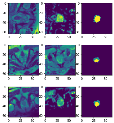
MONAI 1.0 : PyTorch ユーザのための MONAI
このチュートリアルは MONAI API を簡単に紹介してその柔軟性と使い易さにハイライトを当てます。それは PyTorch の基本的な理解を前提とし、MONAI がヘルスケア画像処理における深層学習用にドメインに最適化された機能を提供する方法を示します。
パッケージのインストール
MONAI のコア機能は Python で書かれていて Numpy と Pytorch にのみ依存しています。
このセクションは MONAI の最新版をインストールしてインストールを検証します。
# install the latest weekly preview version of MONAI
%pip install -q "monai-weekly[tqdm, nibabel, gdown, ignite]"
import warnings
warnings.filterwarnings("ignore")  # remove some scikit-image warnings

import monai
monai.config.print_config()
MONAI version: 0.10.dev2237
Numpy version: 1.21.6
Pytorch version: 1.12.1+cu113
MONAI flags: HAS_EXT = False, USE_COMPILED = False, USE_META_DICT = False
MONAI rev id: 533b9b8f56542f7cbca718e062271fd976c267c1
MONAI __file__: /usr/local/lib/python3.7/dist-packages/monai/__init__.py

Optional dependencies:
Pytorch Ignite version: 0.4.10
Nibabel version: 3.0.2
scikit-image version: 0.18.3
Pillow version: 7.1.2
Tensorboard version: 2.8.0
gdown version: 4.4.0
TorchVision version: 0.13.1+cu113
tqdm version: 4.64.1
lmdb version: 0.99
psutil version: 5.4.8
pandas version: 1.3.5
einops version: NOT INSTALLED or UNKNOWN VERSION.
transformers version: NOT INSTALLED or UNKNOWN VERSION.
mlflow version: NOT INSTALLED or UNKNOWN VERSION.
pynrrd version: NOT INSTALLED or UNKNOWN VERSION.

For details about installing the optional dependencies, please visit:
    https://docs.monai.io/en/latest/installation.html#installing-the-recommended-dependencies
数行のコードでパブリックな医用画像データセットへアクセス
公開されているベンチマークの使用はオープンで再現性のある研究のために重要です。MONAI は良く知られた公開データセットへの素早いアクセスを提供することを目的としています。このセクションは医療セグメンテーション・デカスロン (= Medical Segmentation Decathlon ) のデータセットから始めます。
DecathlonDataset オブジェクトは torch.data.utils.Dataset の薄いラッパーです。それは __getitem__ と __len__ を実装していて、PyTorch の組込みデータローダ torch.data.utils.DataLoader と完全に互換です。
PyTorch データセット API と比較して、DecathlonDataset は以下の追加機能を持ちます :
- 自動的なデータのダウンロードと解凍
- データと前処理の中間結果のキャッシング
- 訓練、検証とテストのランダムな分割
from monai.apps import DecathlonDataset

dataset = DecathlonDataset(root_dir="./", task="Task05_Prostate", section="training", transform=None, download=True)
print(f"\nnumber of subjects: {len(dataset)}.\nThe first element in the dataset is {dataset[0]}.")
2022-09-16 06:55:41,150 - INFO - Verified 'Task05_Prostate.tar', md5: 35138f08b1efaef89d7424d2bcc928db.
2022-09-16 06:55:41,152 - INFO - File exists: Task05_Prostate.tar, skipped downloading.
2022-09-16 06:55:41,156 - INFO - Non-empty folder exists in Task05_Prostate, skipped extracting.
Loading dataset: 100%|██████████| 26/26 [00:00<00:00, 186095.40it/s]
number of subjects: 26.
The first element in the dataset is {'image': 'Task05_Prostate/imagesTr/prostate_46.nii.gz', 'label': 'Task05_Prostate/labelsTr/prostate_46.nii.gz'}.
コードセクションは公開レポジトリから "Task05_Prostate.tar" (download=True) をダウンロードして、それを解凍し、そしてアーカイブにより提供される JSON ファイルを解析することにより DecathlonDataset を作成しました。
これは前立腺 (= prostate) 移行 (= transitional) ゾーンと周辺 (= peripheral) ゾーンの輪郭を描く (= delineate) ための 3 クラス・セグメンテーション・タスクです (背景, TZ, PZ クラス)。入力は 2 つの様式、つまり T2 と ADC MRI を持ちます。
len(dataset) と dataset[0] は、それぞれデータセットのサイズを問い合わせ、データセットの最初の要素を取り出します。データセットのためのどのような画像変換も指定していませんので、この iterable なデータセットの出力は画像とセグメンテーション・ファイル名の単なるペアです。
柔軟な画像データ変換
このセクションはファイル名をメモリ内のデータ配列に変換する MONAI 変換を導入します、これにより深層学習モデルにより消費される準備ができます。前処理パイプラインのより多くのサンプルは tutorial レポジトリ と 開発者ガイド で利用可能です。ここでは画像前処理の主要な機能を簡単にカバーします。
配列 vs 辞書ベースの変換
配列変換は MONAI の基本的なビルディングブロックで、それは torchvision.transforms と同様な単純な callable です。2 つの違いがあります :
- MONAI 変換は医用画像特有の処理機能を実装しています。
- MONAI 変換は入力が numpy 配列、pytorch テンソルかテンソル like なオブジェクトであることを前提としています。
以下はローダー変換を開始します、これはファイル名文字列を実際の画像データに変換します。
この変換への より多くのオプションについてのドキュメント を参照してください。
from monai.transforms import LoadImage

loader = LoadImage(image_only=True)
img_array = loader("Task05_Prostate/imagesTr/prostate_02.nii.gz")
print(img_array.shape)
(320, 320, 24, 2)
辞書変換は配列バージョンのラッパーに過ぎません。配列ベースのものと比べて、同じ種類の演算やステートメントを複数のデータ入力に適用することがより簡単です。
以下のセクションは画像とセグメンテーション・マスクのペアを読みます、変換が辞書のどの項目が処理されるべきかを知れるようにキーが指定される必要があることに注意してください。
from monai.transforms import LoadImageD

dict_loader = LoadImageD(keys=("image", "label"))
data_dict = dict_loader({"image": "Task05_Prostate/imagesTr/prostate_02.nii.gz",
                         "label": "Task05_Prostate/labelsTr/prostate_02.nii.gz"})
print(f"image shape: {data_dict['image'].shape}, \nlabel shape: {data_dict['label'].shape}")
image shape: (320, 320, 24, 2),
label shape: (320, 320, 24)
変換の構成
多くの場合、変換のチェインを構築して、前処理パラメータを調整して、高速な前処理パイプラインを作成することは有益です。monai.transforms.Compose はこれらのユースケースのために設計されています。
以下のコードは複数の前処理ステップを行なうために変換チェインを開始しています :
- Nifti 画像を (画像メタデータ情報と共に) ロードします
- 画像とラベルの両方をチャネル first にする (画像を reshape してラベルのためにチャネル次元を追加します)
- 画像とラベルを 1 mm 四方にする
- 画像とラベルの両方を "RAS" 座標系にあるようにする
- 画像強度をスケールする
- 画像とラベルを空間サイズ (64, 64, 32) mm にリサイズする
- 画像をランダムに回転とスケールしますが、出力サイズは (64, 64, 32) mm に保持します。
- 画像とラベルを torch テンソルに変換する
import numpy as np
from monai.transforms import \
    LoadImageD, EnsureChannelFirstD, AddChannelD, ScaleIntensityD, ToTensorD, Compose, \
    AsDiscreteD, SpacingD, OrientationD, ResizeD, RandAffineD
KEYS = ("image", "label")

xform = Compose([
    LoadImageD(KEYS),
    EnsureChannelFirstD("image"),
    AddChannelD("label"),
    OrientationD(KEYS, axcodes='RAS'),
    SpacingD(KEYS, pixdim=(1., 1., 1.), mode=('bilinear', 'nearest')),
    ScaleIntensityD(keys="image"),
    ResizeD(KEYS, (64, 64, 32), mode=('trilinear', 'nearest')),
    RandAffineD(KEYS, spatial_size=(-1, -1, -1),
                rotate_range=(0, 0, np.pi/2),
                scale_range=(0.1, 0.1),
                mode=('bilinear', 'nearest'),
                prob=1.0),
    ToTensorD(KEYS),
])

data_dict = xform({"image": "Task05_Prostate/imagesTr/prostate_02.nii.gz",
                   "label": "Task05_Prostate/labelsTr/prostate_02.nii.gz"})
print(data_dict["image"].shape, data_dict["label"].shape)
(2, 64, 64, 32) (1, 64, 64, 32)
MONAI には有用な変換のセットがあり、今後更に増えます。詳細は https://docs.monai.io/en/latest/transforms.html を見てください。
データセット、変換とデータローダ
私達が持っているものをまとめると :
- Dataset : torch.utils.data.Dataset の薄いラッパー
- Transform : callable、Compose により作成される変換チェインの一部です。
- データセットへの変換のセッティングはデータロードと前処理パイプラインを可能にします。
パイプラインは pytorch ネイティブのデータローダと連携できて、これはマルチプロセッシングのサポートと柔軟なバッチサンプリング・スキームを提供します。
けれども、MONAI データローダ monai.data.DataLoader と連携することが推奨されます、これは pytorch ネイティブのラッパーです。MONAI データローダは以下の機能を主として追加します :
- マルチプロセスのコンテキストでランダム化された増強を正しく処理します。
- マルチサンプルデータのリストを個々の訓練サンプルに平坦化するためのカスタマイズされた collate 関数
DecathlonDataset の初期化は (非ランダム化) 変換結果のキャッシングを含みます。それは遅いかもしれません、複数エポックの訓練のために初期化されたオブジェクトを使用するとき、遥かに改良された速度のために空間を効果的にトレードオフします。
import torch
from monai.data import DataLoader

# start a chain of transforms
xform = Compose([
    LoadImageD(KEYS),
    EnsureChannelFirstD("image"),
    AddChannelD("label"),
    OrientationD(KEYS, axcodes='RAS'),
    SpacingD(KEYS, pixdim=(1., 1., 1.), mode=('bilinear', 'nearest')),
    ScaleIntensityD(keys="image"),
    ResizeD(KEYS, (64, 64, 32), mode=('trilinear', 'nearest')),
    RandAffineD(KEYS, spatial_size=(-1, -1, -1),
                rotate_range=(0, 0, np.pi/2),
                scale_range=(0.1, 0.1),
                mode=('bilinear', 'nearest'),
                prob=1.0),
    ToTensorD(KEYS),
])
# start a dataset
dataset = DecathlonDataset(root_dir="./", task="Task05_Prostate", section="training", transform=xform, download=True)

# start a pytorch dataloader
# data_loader = torch.utils.data.DataLoader(dataset, batch_size=1, shuffle=False, num_workers=1)
data_loader = DataLoader(dataset, batch_size=1, shuffle=True, num_workers=1)
2022-09-16 06:55:43,240 - INFO - Verified 'Task05_Prostate.tar', md5: 35138f08b1efaef89d7424d2bcc928db.
2022-09-16 06:55:43,241 - INFO - File exists: Task05_Prostate.tar, skipped downloading.
2022-09-16 06:55:43,246 - INFO - Non-empty folder exists in Task05_Prostate, skipped extracting.
Loading dataset: 100%|██████████| 26/26 [00:21<00:00,  1.20it/s]
data_dict で何が起きているか覗いてみましょう (以下のセクションの再実行はデータセットからランダムに増強されたサンプルを生成します) :
import matplotlib.pyplot as plt
import numpy as np

data_dict = next(iter(data_loader))
print(data_dict["image"].shape, data_dict["label"].shape, data_dict["image_meta_dict"]["filename_or_obj"])

plt.subplots(1, 3)
plt.subplot(1, 3, 1); plt.imshow(data_dict["image"][0, 0, ..., 16])
plt.subplot(1, 3, 2); plt.imshow(data_dict["image"][0, 1, ..., 16])
plt.subplot(1, 3, 3); plt.imshow(data_dict["label"][0, 0, ..., 16])
plt.show()

print(f"unique labels: {np.unique(data_dict['label'])}")
(1, 2, 64, 64, 32) (1, 1, 64, 64, 32) ['Task05_Prostate/imagesTr/prostate_25.nii.gz']
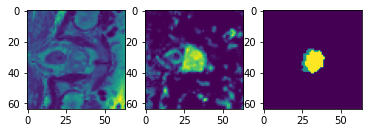
データローダは、深層学習モデルに対応できるように、画像とラベルの両方にバッチ次元を追加しました。
ラベルのために "nearest" 補完モードが使用されますので、変換中に一意のクラスの数が保持されます。
層、ブロック、ネットワークと損失関数
データ入力パイプラインを通り抜けました。適切に前処理されたデータは、2 つの様式の入力を使用して 3 クラス・セグメンテーション・タスクのための準備ができました。
このセクションは UNet モデル、そして損失関数と optimzer を作成します。
これら総てのモジュールは (torch.nn.Module のような) PyTorch インターフェイスの直接的な使用か拡張です。それらは、コードが標準 PyTorch API に従うのであれば、任意のカスタマイズされた Python コードで置き換え可能です。
MONAI のモジュールは医用画像解析のために拡張モジュールを提供することに焦点を当てています :
- 柔軟性とコード可読性の両者を目的とした参照ネットワークの実装
- 1D, 2D と 3D ネットワークと互換な事前定義された層とブロック
- ドメイン固有の損失関数
from monai.networks.nets import UNet
from monai.networks.layers import Norm
from monai.losses import DiceLoss

device = torch.device('cuda:0')
net = UNet(dimensions=3, in_channels=2, out_channels=3, channels=(16, 32, 64, 128, 256),
           strides=(2, 2, 2, 2), num_res_units=2, norm=Norm.BATCH).to(device)
loss = DiceLoss(to_onehot_y=True, softmax=True)
opt = torch.optim.Adam(net.parameters(), 1e-2)
UNet は dimensions パラメータで定義されます。それは Conv1d, Conv2d と Conv3d のような、pytorch API の空間次元の数を指定します。同じ実装で、1D, 2D, 3D とマルチモーダル訓練のために容易に構成できます。
torch.nn.Module の拡張としての UNet は特定の方法で体系化された MONAI ブロックと層のセットです。ブロックと層は、"Conv. + Feature Norm. + Activation" のような一般に使用される組合せのように、再利用可能なサブモジュールとして設計されています。
スライディング・ウィンドウ推論
この一般に使用されるモジュールについて、MONAI は単純な PyTorch ベースの実装を提供します、これはウィンドウサイズと入力モデル (これは torch.nn.Module 実装であり得ます) の仕様だけを必要とします。
以下のデモは、総ての空間位置を通して実行される (40, 40) 空間サイズ・ウィンドウを集約することにより、(1, 1, 200, 200) の入力画像上のスライディング・ウィンドウ推論の toy を示します。
roi_size, sw_batch_size と overlap パラメータをそれらのスライディング・ウィンドウ出力上のインパクトを見るために変更することができます。
from monai.inferers import SlidingWindowInferer

class ToyModel:
    # A simple model generates the output by adding an integer `pred` to input.
    # each call of this instance increases the integer by 1.
    pred = 0
    def __call__(self, input):
        self.pred = self.pred + 1
        input = input + self.pred
        return input

infer = SlidingWindowInferer(roi_size=(40, 40), sw_batch_size=1, overlap=0)
input_tensor = torch.zeros(1, 1, 200, 200)
output_tensor = infer(input_tensor, ToyModel())
plt.imshow(output_tensor[0, 0]); plt.show()
訓練ワークフローの開始 (エポック毎に検証)
入力パイプライン、ネットワーク・アーキテクチャ、損失関数は総て既存の pytorch ベースのワークフローと互換です。様々なユースケースについてはチュートリアルを参照してください : https://github.com/Project-MONAI/tutorials
ここで PyTorch-Ignite ベースで MONAI により構築された、ワークフロー・ユティリティにハイライトを当てたいです。主要な目標は、比較的標準的な訓練ワークフローを構築する際にユーザの労力を軽減することです。
import ignite
print(ignite.__version__)
0.4.10
以下のコマンドは SupervisedTrainer インスタンスを起動します。PyTorch ignite の機能の拡張として、それは前述した総ての要素を結合します。trainer.run() の呼び出しは 2 エポックの間ネットワークを訓練して、総てのエポックの最後に訓練データに基づいて MeadDice メトリックを計算します。
key_train_metric はモデルの品質向上の進捗を追跡するために使用されます。追加のハンドラが早期停止と学習率スケジューリングを行なうために設定できます。
StatsHandler は診断情報を stdout にプリントするために訓練反復毎にトリガーされます。これらはユーザ指定の頻度で詳細な訓練ログを生成するように構成できます。
イベント処理システムの詳細は、ドキュメント https://docs.monai.io/en/latest/handlers.html を参照してください。
注目すべき点は、これらの機能は通常の訓練と検証パイプラインの高速なプロトタイピングを容易にすることです。ユーザは前のセクションで述べたモジュールを利用して、独自のパイプラインを構築することを常に選択できます。
from monai.engines import SupervisedTrainer
from monai.inferers import SlidingWindowInferer
from monai.handlers import StatsHandler, MeanDice, from_engine
from monai.transforms import AsDiscreteD

import sys
import logging
logging.basicConfig(stream=sys.stdout, level=logging.INFO)

trainer = SupervisedTrainer(
    device=device,
    max_epochs=2,
    train_data_loader=data_loader,
    network=net,
    optimizer=opt,
    loss_function=loss,
    inferer=SlidingWindowInferer((32, 32, -1), sw_batch_size=2),
    postprocessing=AsDiscreteD(keys=["pred", "label"], argmax=(True, False), to_onehot=3),
    key_train_metric={"train_meandice": MeanDice(output_transform=from_engine(["pred", "label"]))},
    train_handlers=StatsHandler(tag_name="train_loss", output_transform=from_engine(["loss"], first=True)),
)
trainer.run()
INFO:ignite.engine.engine.SupervisedTrainer:Engine run resuming from iteration 0, epoch 0 until 2 epochs
INFO:ignite.engine.engine.SupervisedTrainer:Epoch: 1/2, Iter: 1/26 -- train_loss: 0.8139
INFO:ignite.engine.engine.SupervisedTrainer:Epoch: 1/2, Iter: 2/26 -- train_loss: 0.7707
INFO:ignite.engine.engine.SupervisedTrainer:Epoch: 1/2, Iter: 3/26 -- train_loss: 0.6901
INFO:ignite.engine.engine.SupervisedTrainer:Epoch: 1/2, Iter: 4/26 -- train_loss: 0.6979
INFO:ignite.engine.engine.SupervisedTrainer:Epoch: 1/2, Iter: 5/26 -- train_loss: 0.7192
INFO:ignite.engine.engine.SupervisedTrainer:Epoch: 1/2, Iter: 6/26 -- train_loss: 0.6859
INFO:ignite.engine.engine.SupervisedTrainer:Epoch: 1/2, Iter: 7/26 -- train_loss: 0.6445
INFO:ignite.engine.engine.SupervisedTrainer:Epoch: 1/2, Iter: 8/26 -- train_loss: 0.6273
INFO:ignite.engine.engine.SupervisedTrainer:Epoch: 1/2, Iter: 9/26 -- train_loss: 0.6346
INFO:ignite.engine.engine.SupervisedTrainer:Epoch: 1/2, Iter: 10/26 -- train_loss: 0.6078
INFO:ignite.engine.engine.SupervisedTrainer:Epoch: 1/2, Iter: 11/26 -- train_loss: 0.5424
INFO:ignite.engine.engine.SupervisedTrainer:Epoch: 1/2, Iter: 12/26 -- train_loss: 0.5851
INFO:ignite.engine.engine.SupervisedTrainer:Epoch: 1/2, Iter: 13/26 -- train_loss: 0.5647
INFO:ignite.engine.engine.SupervisedTrainer:Epoch: 1/2, Iter: 14/26 -- train_loss: 0.5551
INFO:ignite.engine.engine.SupervisedTrainer:Epoch: 1/2, Iter: 15/26 -- train_loss: 0.5925
INFO:ignite.engine.engine.SupervisedTrainer:Epoch: 1/2, Iter: 16/26 -- train_loss: 0.5389
INFO:ignite.engine.engine.SupervisedTrainer:Epoch: 1/2, Iter: 17/26 -- train_loss: 0.5662
INFO:ignite.engine.engine.SupervisedTrainer:Epoch: 1/2, Iter: 18/26 -- train_loss: 0.6309
INFO:ignite.engine.engine.SupervisedTrainer:Epoch: 1/2, Iter: 19/26 -- train_loss: 0.6168
INFO:ignite.engine.engine.SupervisedTrainer:Epoch: 1/2, Iter: 20/26 -- train_loss: 0.5556
INFO:ignite.engine.engine.SupervisedTrainer:Epoch: 1/2, Iter: 21/26 -- train_loss: 0.5243
INFO:ignite.engine.engine.SupervisedTrainer:Epoch: 1/2, Iter: 22/26 -- train_loss: 0.5801
INFO:ignite.engine.engine.SupervisedTrainer:Epoch: 1/2, Iter: 23/26 -- train_loss: 0.5132
INFO:ignite.engine.engine.SupervisedTrainer:Epoch: 1/2, Iter: 24/26 -- train_loss: 0.4951
INFO:ignite.engine.engine.SupervisedTrainer:Epoch: 1/2, Iter: 25/26 -- train_loss: 0.4870
INFO:ignite.engine.engine.SupervisedTrainer:Epoch: 1/2, Iter: 26/26 -- train_loss: 0.5108
INFO:ignite.engine.engine.SupervisedTrainer:Got new best metric of train_meandice: 0.4181462824344635
INFO:ignite.engine.engine.SupervisedTrainer:Epoch[1] Metrics -- train_meandice: 0.4181
INFO:ignite.engine.engine.SupervisedTrainer:Key metric: train_meandice best value: 0.4181462824344635 at epoch: 1
INFO:ignite.engine.engine.SupervisedTrainer:Epoch[1] Complete. Time taken: 00:00:08
INFO:ignite.engine.engine.SupervisedTrainer:Epoch: 2/2, Iter: 1/26 -- train_loss: 0.5620
INFO:ignite.engine.engine.SupervisedTrainer:Epoch: 2/2, Iter: 2/26 -- train_loss: 0.5373
INFO:ignite.engine.engine.SupervisedTrainer:Epoch: 2/2, Iter: 3/26 -- train_loss: 0.4764
INFO:ignite.engine.engine.SupervisedTrainer:Epoch: 2/2, Iter: 4/26 -- train_loss: 0.5111
INFO:ignite.engine.engine.SupervisedTrainer:Epoch: 2/2, Iter: 5/26 -- train_loss: 0.5922
INFO:ignite.engine.engine.SupervisedTrainer:Epoch: 2/2, Iter: 6/26 -- train_loss: 0.5519
INFO:ignite.engine.engine.SupervisedTrainer:Epoch: 2/2, Iter: 7/26 -- train_loss: 0.6246
INFO:ignite.engine.engine.SupervisedTrainer:Epoch: 2/2, Iter: 8/26 -- train_loss: 0.4363
INFO:ignite.engine.engine.SupervisedTrainer:Epoch: 2/2, Iter: 9/26 -- train_loss: 0.5052
INFO:ignite.engine.engine.SupervisedTrainer:Epoch: 2/2, Iter: 10/26 -- train_loss: 0.5900
INFO:ignite.engine.engine.SupervisedTrainer:Epoch: 2/2, Iter: 11/26 -- train_loss: 0.5997
INFO:ignite.engine.engine.SupervisedTrainer:Epoch: 2/2, Iter: 12/26 -- train_loss: 0.4996
INFO:ignite.engine.engine.SupervisedTrainer:Epoch: 2/2, Iter: 13/26 -- train_loss: 0.4969
INFO:ignite.engine.engine.SupervisedTrainer:Epoch: 2/2, Iter: 14/26 -- train_loss: 0.5740
INFO:ignite.engine.engine.SupervisedTrainer:Epoch: 2/2, Iter: 15/26 -- train_loss: 0.5852
INFO:ignite.engine.engine.SupervisedTrainer:Epoch: 2/2, Iter: 16/26 -- train_loss: 0.5460
INFO:ignite.engine.engine.SupervisedTrainer:Epoch: 2/2, Iter: 17/26 -- train_loss: 0.5034
INFO:ignite.engine.engine.SupervisedTrainer:Epoch: 2/2, Iter: 18/26 -- train_loss: 0.5233
INFO:ignite.engine.engine.SupervisedTrainer:Epoch: 2/2, Iter: 19/26 -- train_loss: 0.5109
INFO:ignite.engine.engine.SupervisedTrainer:Epoch: 2/2, Iter: 20/26 -- train_loss: 0.4877
INFO:ignite.engine.engine.SupervisedTrainer:Epoch: 2/2, Iter: 21/26 -- train_loss: 0.5745
INFO:ignite.engine.engine.SupervisedTrainer:Epoch: 2/2, Iter: 22/26 -- train_loss: 0.5044
INFO:ignite.engine.engine.SupervisedTrainer:Epoch: 2/2, Iter: 23/26 -- train_loss: 0.4623
INFO:ignite.engine.engine.SupervisedTrainer:Epoch: 2/2, Iter: 24/26 -- train_loss: 0.4399
INFO:ignite.engine.engine.SupervisedTrainer:Epoch: 2/2, Iter: 25/26 -- train_loss: 0.4553
INFO:ignite.engine.engine.SupervisedTrainer:Epoch: 2/2, Iter: 26/26 -- train_loss: 0.5245
INFO:ignite.engine.engine.SupervisedTrainer:Got new best metric of train_meandice: 0.4688393473625183
INFO:ignite.engine.engine.SupervisedTrainer:Epoch[2] Metrics -- train_meandice: 0.4688
INFO:ignite.engine.engine.SupervisedTrainer:Key metric: train_meandice best value: 0.4688393473625183 at epoch: 2
INFO:ignite.engine.engine.SupervisedTrainer:Epoch[2] Complete. Time taken: 00:00:08
INFO:ignite.engine.engine.SupervisedTrainer:Engine run complete. Time taken: 00:00:16
決定論的訓練
決定論的訓練サポートは再現可能な研究のために重要です。MONAI は現在 2 つのメカニズムを提供しています :
- 総てのランダム変換のランダム状態を設定します。これはグローバルなランダム状態には影響しません。例えば :
# define a transform chain for pre-processing train_transforms = monai.transforms.Compose([ LoadImaged(keys=['image', 'label']), RandRotate90d(keys=['image', 'label'], prob=0.2, spatial_axes=[0, 2]), ... ... ]) # set determinism for reproducibility train_transforms.set_random_state(seed=0) - 1 行のコードでグローバルに python, numpy と pytorch のための決定論的訓練を有効にします、例えば :
monai.utils.set_determinism(seed=0, additional_settings=None)
まとめ
MONAI の主要なモジュールを通り抜けてきました。高度に柔軟な拡張とラッパーを作成することにより、MONAI は医用画像解析の観点から pytorch API を強化しています。
以下のような、この短いチュートリアルではカバーされなかったソフトウェア機能があります :
- 後処理変換
- 視覚化インターフェイス
- サードパーティの医用画像ツールキットからの組み込めるデータ変換
- 他の人気のある深層学習フレームワークを使用するワークフローの構築
- MONAI 研究
最新のマイルストーンのハイライトの詳細については、https://docs.monai.io/en/latest/highlights.html にアクセスしてください。
MONAI を深く理解するには、examples レポジトリは良い開始点です : https://github.com/Project-MONAI/tutorials
API ドキュメントについては、https://docs.monai.io にアクセスしてください。
以上
ClassCat® Chatbot
人工知能開発支援
- テクニカルコンサルティングサービス
- 実証実験 (プロトタイプ構築)
- アプリケーションへの実装
- 人工知能研修サービス
クラスキャット
セールス・インフォメーション
E-Mail:sales-info@classcat.com