ホーム » sales-info の投稿 (ページ 5)
作者アーカイブ: sales-info
MONAI 0.7 : tutorials : 2D 分類 – MedNIST データセットによる医用画像分類
MONAI 0.7 : tutorials : 2D 分類 – MedNIST データセットによる医用画像分類 (翻訳/解説)
翻訳 : (株)クラスキャット セールスインフォメーション
作成日時 : 10/05/2021 (0.7.0)
* 本ページは、MONAI の以下のドキュメントを翻訳した上で適宜、補足説明したものです:
* サンプルコードの動作確認はしておりますが、必要な場合には適宜、追加改変しています。
* ご自由にリンクを張って頂いてかまいませんが、sales-info@classcat.com までご一報いただけると嬉しいです。

- 人工知能研究開発支援
- 人工知能研修サービス(経営者層向けオンサイト研修)
- テクニカルコンサルティングサービス
- 実証実験(プロトタイプ構築)
- アプリケーションへの実装
- 人工知能研修サービス
- PoC(概念実証)を失敗させないための支援
- テレワーク & オンライン授業を支援
- お住まいの地域に関係なく Web ブラウザからご参加頂けます。事前登録 が必要ですのでご注意ください。
- ウェビナー運用には弊社製品「ClassCat® Webinar」を利用しています。
◆ お問合せ : 本件に関するお問い合わせ先は下記までお願いいたします。
| 株式会社クラスキャット セールス・マーケティング本部 セールス・インフォメーション |
| E-Mail:sales-info@classcat.com ; WebSite: https://www.classcat.com/ ; Facebook |
MONAI 0.7 : tutorials : 2D 分類 – MedNIST データセットによる医用画像分類
このノートブックは MONAI 機能を既存の PyTorch プログラムに容易に統合する方法を示します。それは MedNIST データセットに基づいています、これは初心者のためにチュートリアルとして非常に適切です。このチュートリアルはまた MONAI 組込みのオクルージョン感度の機能も利用しています。
また、このチュートリアルでは、MONAIに内蔵されているオクルージョン感度機能も利用しています。
このチュートリアルでは、MedNIST データセットに基づく end-to-end な訓練と評価サンプルを紹介します。
以下のステップで進めます :
- 訓練とテストのためにデータセットを作成する。
- データを前処理するために MONAI 変換を利用します。
- 分類のために MONAI から DenseNet を利用します。
- モデルを PyTorch プログラムで訓練します。
- テストデータセット上で評価します。
環境のセットアップ
!python -c "import monai" || pip install -q "monai-weekly[pillow, tqdm]"
!python -c "import matplotlib" || pip install -q matplotlib
%matplotlib inline
インポートのセットアップ
# Copyright 2020 MONAI Consortium
# Licensed under the Apache License, Version 2.0 (the "License");
# you may not use this file except in compliance with the License.
# You may obtain a copy of the License at
#     http://www.apache.org/licenses/LICENSE-2.0
# Unless required by applicable law or agreed to in writing, software
# distributed under the License is distributed on an "AS IS" BASIS,
# WITHOUT WARRANTIES OR CONDITIONS OF ANY KIND, either express or implied.
# See the License for the specific language governing permissions and
# limitations under the License.

import os
import shutil
import tempfile
import matplotlib.pyplot as plt
import PIL
import torch
import numpy as np
from sklearn.metrics import classification_report

from monai.apps import download_and_extract
from monai.config import print_config
from monai.data import decollate_batch
from monai.metrics import ROCAUCMetric
from monai.networks.nets import DenseNet121
from monai.transforms import (
    Activations,
    AddChannel,
    AsDiscrete,
    Compose,
    LoadImage,
    RandFlip,
    RandRotate,
    RandZoom,
    ScaleIntensity,
    EnsureType,
)
from monai.utils import set_determinism

print_config()
MONAI version: 0.6.0rc1+15.gf3d436a0
Numpy version: 1.20.3
Pytorch version: 1.9.0a0+c3d40fd
MONAI flags: HAS_EXT = True, USE_COMPILED = False
MONAI rev id: f3d436a09deefcf905ece2faeec37f55ab030003

Optional dependencies:
Pytorch Ignite version: 0.4.5
Nibabel version: 3.2.1
scikit-image version: 0.15.0
Pillow version: 8.2.0
Tensorboard version: 2.5.0
gdown version: 3.13.0
TorchVision version: 0.10.0a0
ITK version: 5.1.2
tqdm version: 4.53.0
lmdb version: 1.2.1
psutil version: 5.8.0
pandas version: 1.1.4
einops version: 0.3.0

For details about installing the optional dependencies, please visit:
    https://docs.monai.io/en/latest/installation.html#installing-the-recommended-dependencies
データディレクトリのセットアップ
MONAI_DATA_DIRECTORY 環境変数でディレクトリを指定できます。これは結果をセーブしてダウンロードを再利用することを可能にします。指定されない場合、一時ディレクトリが使用されます。
directory = os.environ.get("MONAI_DATA_DIRECTORY")
root_dir = tempfile.mkdtemp() if directory is None else directory
print(root_dir)
/workspace/data/medical
データセットをダウンロードする
MedMNIST データセットは TCIA, RSNA Bone Age チャレンジ と NIH Chest X-ray データセット からの様々なセットから集められました。
データセットは Dr. Bradley J. Erickson M.D., Ph.D. (Department of Radiology, Mayo Clinic) のお陰により Creative Commons CC BY-SA 4.0 ライセンス のもとで利用可能になっています。
MedNIST データセットを使用する場合、出典を明示してください。
resource = "https://drive.google.com/uc?id=1QsnnkvZyJPcbRoV_ArW8SnE1OTuoVbKE"
md5 = "0bc7306e7427e00ad1c5526a6677552d"

compressed_file = os.path.join(root_dir, "MedNIST.tar.gz")
data_dir = os.path.join(root_dir, "MedNIST")
if not os.path.exists(data_dir):
    download_and_extract(resource, compressed_file, root_dir, md5)
再現性のために決定論的訓練を設定する
set_determinism(seed=0)
データセットフォルダから画像ファイル名を読む
まず最初に、データセットファイルを確認して幾つかの統計を表示します。
データセットには 6 つのフォルダがあります : Hand, AbdomenCT, CXR, ChestCT, BreastMRI, HeadCT,
これらは分類モデルを訓練するためにラベルとして使用されるべきです。
class_names = sorted(x for x in os.listdir(data_dir)
                     if os.path.isdir(os.path.join(data_dir, x)))
num_class = len(class_names)
image_files = [
    [
        os.path.join(data_dir, class_names[i], x)
        for x in os.listdir(os.path.join(data_dir, class_names[i]))
    ]
    for i in range(num_class)
]
num_each = [len(image_files[i]) for i in range(num_class)]
image_files_list = []
image_class = []
for i in range(num_class):
    image_files_list.extend(image_files[i])
    image_class.extend([i] * num_each[i])
num_total = len(image_class)
image_width, image_height = PIL.Image.open(image_files_list[0]).size

print(f"Total image count: {num_total}")
print(f"Image dimensions: {image_width} x {image_height}")
print(f"Label names: {class_names}")
print(f"Label counts: {num_each}")
Total image count: 58954
Image dimensions: 64 x 64
Label names: ['AbdomenCT', 'BreastMRI', 'CXR', 'ChestCT', 'Hand', 'HeadCT']
Label counts: [10000, 8954, 10000, 10000, 10000, 10000]
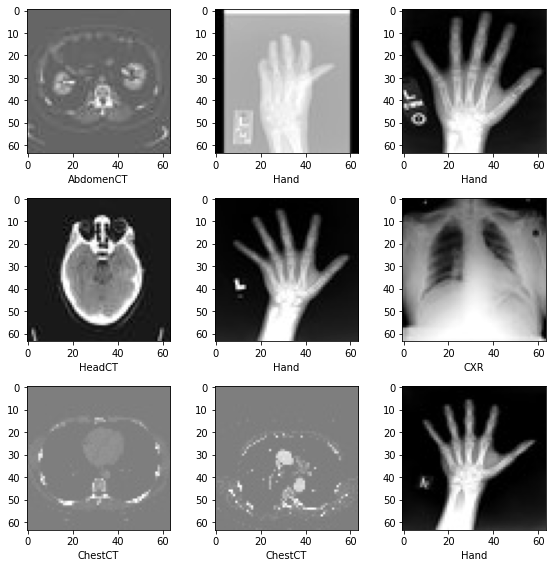
データセットから画像をランダムに選択して可視化して確認する
plt.subplots(3, 3, figsize=(8, 8))
for i, k in enumerate(np.random.randint(num_total, size=9)):
    im = PIL.Image.open(image_files_list[k])
    arr = np.array(im)
    plt.subplot(3, 3, i + 1)
    plt.xlabel(class_names[image_class[k]])
    plt.imshow(arr, cmap="gray", vmin=0, vmax=255)
plt.tight_layout()
plt.show()
訓練、検証とテストデータのリストを準備する
データセットの 10% を検証用に、そして 10% をテスト用にランダムに選択します。
val_frac = 0.1
test_frac = 0.1
length = len(image_files_list)
indices = np.arange(length)
np.random.shuffle(indices)

test_split = int(test_frac * length)
val_split = int(val_frac * length) + test_split
test_indices = indices[:test_split]
val_indices = indices[test_split:val_split]
train_indices = indices[val_split:]

train_x = [image_files_list[i] for i in train_indices]
train_y = [image_class[i] for i in train_indices]
val_x = [image_files_list[i] for i in val_indices]
val_y = [image_class[i] for i in val_indices]
test_x = [image_files_list[i] for i in test_indices]
test_y = [image_class[i] for i in test_indices]

print(
    f"Training count: {len(train_x)}, Validation count: "
    f"{len(val_x)}, Test count: {len(test_x)}")
Training count: 47156, Validation count: 5913, Test count: 5885
データを前処理するために MONAI 変換、Dataset と Dataloader を定義する
train_transforms = Compose(
    [
        LoadImage(image_only=True),
        AddChannel(),
        ScaleIntensity(),
        RandRotate(range_x=np.pi / 12, prob=0.5, keep_size=True),
        RandFlip(spatial_axis=0, prob=0.5),
        RandZoom(min_zoom=0.9, max_zoom=1.1, prob=0.5),
        EnsureType(),
    ]
)

val_transforms = Compose(
    [LoadImage(image_only=True), AddChannel(), ScaleIntensity(), EnsureType()])

y_pred_trans = Compose([EnsureType(), Activations(softmax=True)])
y_trans = Compose([EnsureType(), AsDiscrete(to_onehot=True, num_classes=num_class)])
class MedNISTDataset(torch.utils.data.Dataset):
    def __init__(self, image_files, labels, transforms):
        self.image_files = image_files
        self.labels = labels
        self.transforms = transforms

    def __len__(self):
        return len(self.image_files)

    def __getitem__(self, index):
        return self.transforms(self.image_files[index]), self.labels[index]


train_ds = MedNISTDataset(train_x, train_y, train_transforms)
train_loader = torch.utils.data.DataLoader(
    train_ds, batch_size=300, shuffle=True, num_workers=10)

val_ds = MedNISTDataset(val_x, val_y, val_transforms)
val_loader = torch.utils.data.DataLoader(
    val_ds, batch_size=300, num_workers=10)

test_ds = MedNISTDataset(test_x, test_y, val_transforms)
test_loader = torch.utils.data.DataLoader(
    test_ds, batch_size=300, num_workers=10)
ネットワークと optimizer を定義する
- バッチ毎にモデルがどのくらい更新されるかについて学習率を設定します。
- 合計エポック数を設定します、シャッフルしてランダムな変換を行ないますので、総てのエポックの訓練データは異なります。そしてこれは get start チュートリアルに過ぎませんので、4 エポックだけ訓練しましょう。10 エポック訓練すれば、モデルはテストデータセット上で 100% 精度を達成できます。
- MONAI からの DenseNet を使用して GPU デバイスに移動します、この DenseNet は 2D と 3D 分類タスクの両方をサポートできます。
- Adam optimizer を使用します。
device = torch.device("cuda" if torch.cuda.is_available() else "cpu")
model = DenseNet121(spatial_dims=2, in_channels=1,
                    out_channels=num_class).to(device)
loss_function = torch.nn.CrossEntropyLoss()
optimizer = torch.optim.Adam(model.parameters(), 1e-5)
max_epochs = 4
val_interval = 1
auc_metric = ROCAUCMetric()
モデル訓練
典型的な PyTorch 訓練を実行します、これはエポック・ループとステップ・ループを実行して、総てのエポック後に検証を行ないます。ベストの検証精度を得た場合、モデル重みをファイルにセーブします。
best_metric = -1
best_metric_epoch = -1
epoch_loss_values = []
metric_values = []

for epoch in range(max_epochs):
    print("-" * 10)
    print(f"epoch {epoch + 1}/{max_epochs}")
    model.train()
    epoch_loss = 0
    step = 0
    for batch_data in train_loader:
        step += 1
        inputs, labels = batch_data[0].to(device), batch_data[1].to(device)
        optimizer.zero_grad()
        outputs = model(inputs)
        loss = loss_function(outputs, labels)
        loss.backward()
        optimizer.step()
        epoch_loss += loss.item()
        print(
            f"{step}/{len(train_ds) // train_loader.batch_size}, "
            f"train_loss: {loss.item():.4f}")
        epoch_len = len(train_ds) // train_loader.batch_size
    epoch_loss /= step
    epoch_loss_values.append(epoch_loss)
    print(f"epoch {epoch + 1} average loss: {epoch_loss:.4f}")

    if (epoch + 1) % val_interval == 0:
        model.eval()
        with torch.no_grad():
            y_pred = torch.tensor([], dtype=torch.float32, device=device)
            y = torch.tensor([], dtype=torch.long, device=device)
            for val_data in val_loader:
                val_images, val_labels = (
                    val_data[0].to(device),
                    val_data[1].to(device),
                )
                y_pred = torch.cat([y_pred, model(val_images)], dim=0)
                y = torch.cat([y, val_labels], dim=0)
            y_onehot = [y_trans(i) for i in decollate_batch(y)]
            y_pred_act = [y_pred_trans(i) for i in decollate_batch(y_pred)]
            auc_metric(y_pred_act, y_onehot)
            result = auc_metric.aggregate()
            auc_metric.reset()
            del y_pred_act, y_onehot
            metric_values.append(result)
            acc_value = torch.eq(y_pred.argmax(dim=1), y)
            acc_metric = acc_value.sum().item() / len(acc_value)
            if result > best_metric:
                best_metric = result
                best_metric_epoch = epoch + 1
                torch.save(model.state_dict(), os.path.join(
                    root_dir, "best_metric_model.pth"))
                print("saved new best metric model")
            print(
                f"current epoch: {epoch + 1} current AUC: {result:.4f}"
                f" current accuracy: {acc_metric:.4f}"
                f" best AUC: {best_metric:.4f}"
                f" at epoch: {best_metric_epoch}"
            )

print(
    f"train completed, best_metric: {best_metric:.4f} "
    f"at epoch: {best_metric_epoch}")
---------- epoch 1/4 1/157, train_loss: 1.7898 2/157, train_loss: 1.7560 3/157, train_loss: 1.7461 4/157, train_loss: 1.7241 5/157, train_loss: 1.6973 6/157, train_loss: 1.6706 7/157, train_loss: 1.6388 8/157, train_loss: 1.6210 9/157, train_loss: 1.5989 10/157, train_loss: 1.5599 11/157, train_loss: 1.5826 12/157, train_loss: 1.5339 13/157, train_loss: 1.5235 14/157, train_loss: 1.5098 15/157, train_loss: 1.4746 16/157, train_loss: 1.4584 17/157, train_loss: 1.4365 18/157, train_loss: 1.4328 19/157, train_loss: 1.4274 20/157, train_loss: 1.4327 21/157, train_loss: 1.4017 22/157, train_loss: 1.3231 23/157, train_loss: 1.3180 24/157, train_loss: 1.3001 25/157, train_loss: 1.2958 26/157, train_loss: 1.3021 27/157, train_loss: 1.2336 28/157, train_loss: 1.2154 29/157, train_loss: 1.2595 30/157, train_loss: 1.2050 31/157, train_loss: 1.2161 32/157, train_loss: 1.2106 33/157, train_loss: 1.1495 34/157, train_loss: 1.1550 35/157, train_loss: 1.1246 36/157, train_loss: 1.1607 37/157, train_loss: 1.1126 38/157, train_loss: 1.0987 39/157, train_loss: 1.0694 40/157, train_loss: 1.1181 41/157, train_loss: 1.0576 42/157, train_loss: 1.0703 43/157, train_loss: 1.0414 44/157, train_loss: 1.0446 45/157, train_loss: 1.0313 46/157, train_loss: 0.9786 47/157, train_loss: 0.9767 48/157, train_loss: 0.9579 49/157, train_loss: 0.9659 50/157, train_loss: 1.0069 51/157, train_loss: 0.9868 52/157, train_loss: 0.9637 53/157, train_loss: 0.9301 54/157, train_loss: 0.9382 55/157, train_loss: 0.8923 56/157, train_loss: 0.9034 57/157, train_loss: 0.8674 58/157, train_loss: 0.8707 59/157, train_loss: 0.8876 60/157, train_loss: 0.8628 61/157, train_loss: 0.7709 62/157, train_loss: 0.8494 63/157, train_loss: 0.8264 64/157, train_loss: 0.8011 65/157, train_loss: 0.8186 66/157, train_loss: 0.8016 67/157, train_loss: 0.7813 68/157, train_loss: 0.7447 69/157, train_loss: 0.7201 70/157, train_loss: 0.7323 71/157, train_loss: 0.7332 72/157, train_loss: 0.7379 73/157, train_loss: 0.7495 74/157, train_loss: 0.7157 75/157, train_loss: 0.7007 76/157, train_loss: 0.7058 77/157, train_loss: 0.6814 78/157, train_loss: 0.6738 79/157, train_loss: 0.6449 80/157, train_loss: 0.6393 81/157, train_loss: 0.6238 82/157, train_loss: 0.6234 83/157, train_loss: 0.6262 84/157, train_loss: 0.6044 85/157, train_loss: 0.6005 86/157, train_loss: 0.5783 87/157, train_loss: 0.5570 88/157, train_loss: 0.5569 89/157, train_loss: 0.5633 90/157, train_loss: 0.5199 91/157, train_loss: 0.5846 92/157, train_loss: 0.5915 93/157, train_loss: 0.5612 94/157, train_loss: 0.5785 95/157, train_loss: 0.5654 96/157, train_loss: 0.5437 97/157, train_loss: 0.5429 98/157, train_loss: 0.5053 99/157, train_loss: 0.5221 100/157, train_loss: 0.4928 101/157, train_loss: 0.5064 102/157, train_loss: 0.5104 103/157, train_loss: 0.4830 104/157, train_loss: 0.4901 105/157, train_loss: 0.4957 106/157, train_loss: 0.4913 107/157, train_loss: 0.4722 108/157, train_loss: 0.4756 109/157, train_loss: 0.4803 110/157, train_loss: 0.4534 111/157, train_loss: 0.4383 112/157, train_loss: 0.4437 113/157, train_loss: 0.4264 114/157, train_loss: 0.4067 115/157, train_loss: 0.4268 116/157, train_loss: 0.4136 117/157, train_loss: 0.4115 118/157, train_loss: 0.4082 119/157, train_loss: 0.4246 120/157, train_loss: 0.4018 121/157, train_loss: 0.4161 122/157, train_loss: 0.3475 123/157, train_loss: 0.4233 124/157, train_loss: 0.4043 125/157, train_loss: 0.3192 126/157, train_loss: 0.3611 127/157, train_loss: 0.3475 128/157, train_loss: 0.3580 129/157, train_loss: 0.3286 130/157, train_loss: 0.3688 131/157, train_loss: 0.3205 132/157, train_loss: 0.3745 133/157, train_loss: 0.3709 134/157, train_loss: 0.3535 135/157, train_loss: 0.3729 136/157, train_loss: 0.2839 137/157, train_loss: 0.3614 138/157, train_loss: 0.2981 139/157, train_loss: 0.3280 140/157, train_loss: 0.3031 141/157, train_loss: 0.2994 142/157, train_loss: 0.3296 143/157, train_loss: 0.3032 144/157, train_loss: 0.2965 145/157, train_loss: 0.2955 146/157, train_loss: 0.3379 147/157, train_loss: 0.3339 148/157, train_loss: 0.3092 149/157, train_loss: 0.2723 150/157, train_loss: 0.3171 151/157, train_loss: 0.2933 152/157, train_loss: 0.2841 153/157, train_loss: 0.2723 154/157, train_loss: 0.2954 155/157, train_loss: 0.2955 156/157, train_loss: 0.2969 157/157, train_loss: 0.2674 158/157, train_loss: 0.2465 epoch 1 average loss: 0.7768 saved new best metric model current epoch: 1 current AUC: 0.9984 current accuracy: 0.9618 best AUC: 0.9984 at epoch: 1 ---------- epoch 2/4 1/157, train_loss: 0.2618 2/157, train_loss: 0.2525 3/157, train_loss: 0.2640 4/157, train_loss: 0.2566 5/157, train_loss: 0.2526 6/157, train_loss: 0.2337 7/157, train_loss: 0.2311 8/157, train_loss: 0.2351 9/157, train_loss: 0.2332 10/157, train_loss: 0.2783 11/157, train_loss: 0.2521 12/157, train_loss: 0.2458 13/157, train_loss: 0.2261 14/157, train_loss: 0.2362 15/157, train_loss: 0.2702 16/157, train_loss: 0.2399 17/157, train_loss: 0.2113 18/157, train_loss: 0.2452 19/157, train_loss: 0.2202 20/157, train_loss: 0.2124 21/157, train_loss: 0.2050 22/157, train_loss: 0.2297 23/157, train_loss: 0.2410 24/157, train_loss: 0.2254 25/157, train_loss: 0.2276 26/157, train_loss: 0.2344 27/157, train_loss: 0.1969 28/157, train_loss: 0.2110 29/157, train_loss: 0.2114 30/157, train_loss: 0.2424 31/157, train_loss: 0.2111 32/157, train_loss: 0.1963 33/157, train_loss: 0.1799 34/157, train_loss: 0.1925 35/157, train_loss: 0.2277 36/157, train_loss: 0.2327 37/157, train_loss: 0.1968 38/157, train_loss: 0.2165 39/157, train_loss: 0.1924 40/157, train_loss: 0.1959 41/157, train_loss: 0.1764 42/157, train_loss: 0.2327 43/157, train_loss: 0.1955 44/157, train_loss: 0.1669 45/157, train_loss: 0.1829 46/157, train_loss: 0.1894 47/157, train_loss: 0.2079 48/157, train_loss: 0.1984 49/157, train_loss: 0.2035 50/157, train_loss: 0.1879 51/157, train_loss: 0.1839 52/157, train_loss: 0.1885 53/157, train_loss: 0.1887 54/157, train_loss: 0.1733 55/157, train_loss: 0.1828 56/157, train_loss: 0.1593 57/157, train_loss: 0.1906 58/157, train_loss: 0.1494 59/157, train_loss: 0.1740 60/157, train_loss: 0.1791 61/157, train_loss: 0.1763 62/157, train_loss: 0.1659 63/157, train_loss: 0.1961 64/157, train_loss: 0.1593 65/157, train_loss: 0.1468 66/157, train_loss: 0.1576 67/157, train_loss: 0.1567 68/157, train_loss: 0.1751 69/157, train_loss: 0.1640 70/157, train_loss: 0.1702 71/157, train_loss: 0.1406 72/157, train_loss: 0.1519 73/157, train_loss: 0.1552 74/157, train_loss: 0.1581 75/157, train_loss: 0.1564 76/157, train_loss: 0.1741 77/157, train_loss: 0.1474 78/157, train_loss: 0.1473 79/157, train_loss: 0.1402 80/157, train_loss: 0.1402 81/157, train_loss: 0.1471 82/157, train_loss: 0.1556 83/157, train_loss: 0.1329 84/157, train_loss: 0.1578 85/157, train_loss: 0.1364 86/157, train_loss: 0.1413 87/157, train_loss: 0.1170 88/157, train_loss: 0.1332 89/157, train_loss: 0.1369 90/157, train_loss: 0.1500 91/157, train_loss: 0.1320 92/157, train_loss: 0.1265 93/157, train_loss: 0.1444 94/157, train_loss: 0.1278 95/157, train_loss: 0.1348 96/157, train_loss: 0.1403 97/157, train_loss: 0.1246 98/157, train_loss: 0.1125 99/157, train_loss: 0.1509 100/157, train_loss: 0.1270 101/157, train_loss: 0.1286 102/157, train_loss: 0.1160 103/157, train_loss: 0.1239 104/157, train_loss: 0.1052 105/157, train_loss: 0.1238 106/157, train_loss: 0.1110 107/157, train_loss: 0.1429 108/157, train_loss: 0.1097 109/157, train_loss: 0.1099 110/157, train_loss: 0.1403 111/157, train_loss: 0.1460 112/157, train_loss: 0.1216 113/157, train_loss: 0.1079 114/157, train_loss: 0.1187 115/157, train_loss: 0.1519 116/157, train_loss: 0.1128 117/157, train_loss: 0.1174 118/157, train_loss: 0.1094 119/157, train_loss: 0.1106 120/157, train_loss: 0.1179 121/157, train_loss: 0.1278 122/157, train_loss: 0.1331 123/157, train_loss: 0.1484 124/157, train_loss: 0.1140 125/157, train_loss: 0.1302 126/157, train_loss: 0.1201 127/157, train_loss: 0.1038 128/157, train_loss: 0.1108 129/157, train_loss: 0.1446 130/157, train_loss: 0.0905 131/157, train_loss: 0.1323 132/157, train_loss: 0.0995 133/157, train_loss: 0.0998 134/157, train_loss: 0.0937 135/157, train_loss: 0.1240 136/157, train_loss: 0.0871 137/157, train_loss: 0.1131 138/157, train_loss: 0.1349 139/157, train_loss: 0.1316 140/157, train_loss: 0.0989 141/157, train_loss: 0.1081 142/157, train_loss: 0.1240 143/157, train_loss: 0.1104 144/157, train_loss: 0.0980 145/157, train_loss: 0.1081 146/157, train_loss: 0.0906 147/157, train_loss: 0.1624 148/157, train_loss: 0.1025 149/157, train_loss: 0.1071 150/157, train_loss: 0.0988 151/157, train_loss: 0.1151 152/157, train_loss: 0.1425 153/157, train_loss: 0.1092 154/157, train_loss: 0.0831 155/157, train_loss: 0.1252 156/157, train_loss: 0.0960 157/157, train_loss: 0.1076 158/157, train_loss: 0.0725 epoch 2 average loss: 0.1612 saved new best metric model current epoch: 2 current AUC: 0.9997 current accuracy: 0.9863 best AUC: 0.9997 at epoch: 2 ---------- epoch 3/4 1/157, train_loss: 0.1095 2/157, train_loss: 0.0810 3/157, train_loss: 0.1085 4/157, train_loss: 0.1033 5/157, train_loss: 0.1527 6/157, train_loss: 0.0988 7/157, train_loss: 0.0935 8/157, train_loss: 0.0903 9/157, train_loss: 0.0941 10/157, train_loss: 0.0742 11/157, train_loss: 0.1127 12/157, train_loss: 0.0803 13/157, train_loss: 0.0937 14/157, train_loss: 0.0810 15/157, train_loss: 0.0965 16/157, train_loss: 0.0705 17/157, train_loss: 0.0802 18/157, train_loss: 0.1040 19/157, train_loss: 0.0940 20/157, train_loss: 0.0758 21/157, train_loss: 0.1002 22/157, train_loss: 0.0720 23/157, train_loss: 0.0773 24/157, train_loss: 0.0906 25/157, train_loss: 0.1002 26/157, train_loss: 0.0948 27/157, train_loss: 0.0731 28/157, train_loss: 0.0938 29/157, train_loss: 0.0731 30/157, train_loss: 0.1004 31/157, train_loss: 0.0829 32/157, train_loss: 0.0864 33/157, train_loss: 0.0729 34/157, train_loss: 0.0773 35/157, train_loss: 0.0719 36/157, train_loss: 0.0875 37/157, train_loss: 0.0897 38/157, train_loss: 0.0740 39/157, train_loss: 0.1091 40/157, train_loss: 0.0652 41/157, train_loss: 0.0899 42/157, train_loss: 0.0853 43/157, train_loss: 0.0727 44/157, train_loss: 0.0843 45/157, train_loss: 0.0878 46/157, train_loss: 0.1135 47/157, train_loss: 0.1041 48/157, train_loss: 0.0935 49/157, train_loss: 0.0879 50/157, train_loss: 0.0922 51/157, train_loss: 0.0862 52/157, train_loss: 0.0692 53/157, train_loss: 0.0784 54/157, train_loss: 0.0986 55/157, train_loss: 0.0707 56/157, train_loss: 0.1013 57/157, train_loss: 0.0598 58/157, train_loss: 0.0639 59/157, train_loss: 0.0587 60/157, train_loss: 0.1027 61/157, train_loss: 0.0711 62/157, train_loss: 0.0775 63/157, train_loss: 0.1045 64/157, train_loss: 0.0655 65/157, train_loss: 0.0621 66/157, train_loss: 0.0636 67/157, train_loss: 0.0774 68/157, train_loss: 0.0875 69/157, train_loss: 0.0664 70/157, train_loss: 0.0707 71/157, train_loss: 0.0814 72/157, train_loss: 0.1022 73/157, train_loss: 0.0820 74/157, train_loss: 0.0829 75/157, train_loss: 0.0809 76/157, train_loss: 0.0975 77/157, train_loss: 0.0684 78/157, train_loss: 0.0686 79/157, train_loss: 0.0831 80/157, train_loss: 0.0671 81/157, train_loss: 0.0647 82/157, train_loss: 0.0574 83/157, train_loss: 0.0611 84/157, train_loss: 0.0886 85/157, train_loss: 0.0674 86/157, train_loss: 0.0609 87/157, train_loss: 0.0582 88/157, train_loss: 0.0584 89/157, train_loss: 0.0751 90/157, train_loss: 0.0720 91/157, train_loss: 0.0727 92/157, train_loss: 0.0664 93/157, train_loss: 0.0681 94/157, train_loss: 0.0791 95/157, train_loss: 0.0880 96/157, train_loss: 0.0746 97/157, train_loss: 0.0730 98/157, train_loss: 0.0818 99/157, train_loss: 0.0617 100/157, train_loss: 0.0646 101/157, train_loss: 0.0607 102/157, train_loss: 0.0749 103/157, train_loss: 0.0656 104/157, train_loss: 0.0607 105/157, train_loss: 0.0713 106/157, train_loss: 0.0725 107/157, train_loss: 0.0711 108/157, train_loss: 0.0642 109/157, train_loss: 0.0624 110/157, train_loss: 0.0685 111/157, train_loss: 0.0542 112/157, train_loss: 0.0771 113/157, train_loss: 0.0786 114/157, train_loss: 0.0580 115/157, train_loss: 0.0698 116/157, train_loss: 0.0847 117/157, train_loss: 0.0542 118/157, train_loss: 0.0760 119/157, train_loss: 0.0817 120/157, train_loss: 0.0904 121/157, train_loss: 0.0705 122/157, train_loss: 0.0541 123/157, train_loss: 0.0521 124/157, train_loss: 0.0555 125/157, train_loss: 0.0491 126/157, train_loss: 0.0504 127/157, train_loss: 0.0598 128/157, train_loss: 0.0417 129/157, train_loss: 0.0470 130/157, train_loss: 0.0584 131/157, train_loss: 0.0498 132/157, train_loss: 0.0532 133/157, train_loss: 0.0515 134/157, train_loss: 0.0575 135/157, train_loss: 0.0506 136/157, train_loss: 0.0519 137/157, train_loss: 0.0727 138/157, train_loss: 0.0796 139/157, train_loss: 0.0469 140/157, train_loss: 0.0509 141/157, train_loss: 0.0501 142/157, train_loss: 0.0603 143/157, train_loss: 0.0499 144/157, train_loss: 0.0585 145/157, train_loss: 0.0590 146/157, train_loss: 0.0447 147/157, train_loss: 0.0699 148/157, train_loss: 0.0595 149/157, train_loss: 0.0372 150/157, train_loss: 0.0446 151/157, train_loss: 0.0576 152/157, train_loss: 0.0735 153/157, train_loss: 0.0464 154/157, train_loss: 0.0742 155/157, train_loss: 0.0356 156/157, train_loss: 0.0492 157/157, train_loss: 0.0644 158/157, train_loss: 0.0630 epoch 3 average loss: 0.0743 saved new best metric model current epoch: 3 current AUC: 0.9999 current accuracy: 0.9924 best AUC: 0.9999 at epoch: 3 ---------- epoch 4/4 1/157, train_loss: 0.0563 2/157, train_loss: 0.0645 3/157, train_loss: 0.0497 4/157, train_loss: 0.0579 5/157, train_loss: 0.0442 6/157, train_loss: 0.0588 7/157, train_loss: 0.0501 8/157, train_loss: 0.0402 9/157, train_loss: 0.0432 10/157, train_loss: 0.0465 11/157, train_loss: 0.0546 12/157, train_loss: 0.0548 13/157, train_loss: 0.0430 14/157, train_loss: 0.0448 15/157, train_loss: 0.0533 16/157, train_loss: 0.0521 17/157, train_loss: 0.0406 18/157, train_loss: 0.0426 19/157, train_loss: 0.0471 20/157, train_loss: 0.0570 21/157, train_loss: 0.0611 22/157, train_loss: 0.0500 23/157, train_loss: 0.0532 24/157, train_loss: 0.0549 25/157, train_loss: 0.0488 26/157, train_loss: 0.0574 27/157, train_loss: 0.0587 28/157, train_loss: 0.0488 29/157, train_loss: 0.0509 30/157, train_loss: 0.0299 31/157, train_loss: 0.0404 32/157, train_loss: 0.0345 33/157, train_loss: 0.0569 34/157, train_loss: 0.0361 35/157, train_loss: 0.0623 36/157, train_loss: 0.0686 37/157, train_loss: 0.0376 38/157, train_loss: 0.0528 39/157, train_loss: 0.0367 40/157, train_loss: 0.0466 41/157, train_loss: 0.0551 42/157, train_loss: 0.0374 43/157, train_loss: 0.0681 44/157, train_loss: 0.0386 45/157, train_loss: 0.0636 46/157, train_loss: 0.0555 47/157, train_loss: 0.0449 48/157, train_loss: 0.0481 49/157, train_loss: 0.0382 50/157, train_loss: 0.0682 51/157, train_loss: 0.0511 52/157, train_loss: 0.0606 53/157, train_loss: 0.0490 54/157, train_loss: 0.0497 55/157, train_loss: 0.0476 56/157, train_loss: 0.0457 57/157, train_loss: 0.0545 58/157, train_loss: 0.0426 59/157, train_loss: 0.0445 60/157, train_loss: 0.0528 61/157, train_loss: 0.0597 62/157, train_loss: 0.0376 63/157, train_loss: 0.0555 64/157, train_loss: 0.0571 65/157, train_loss: 0.0475 66/157, train_loss: 0.0577 67/157, train_loss: 0.0393 68/157, train_loss: 0.0397 69/157, train_loss: 0.0536 70/157, train_loss: 0.0516 71/157, train_loss: 0.0595 72/157, train_loss: 0.0473 73/157, train_loss: 0.0624 74/157, train_loss: 0.0426 75/157, train_loss: 0.0474 76/157, train_loss: 0.0474 77/157, train_loss: 0.0516 78/157, train_loss: 0.0332 79/157, train_loss: 0.0403 80/157, train_loss: 0.0401 81/157, train_loss: 0.0397 82/157, train_loss: 0.0526 83/157, train_loss: 0.0429 84/157, train_loss: 0.0306 85/157, train_loss: 0.0433 86/157, train_loss: 0.0376 87/157, train_loss: 0.0430 88/157, train_loss: 0.0433 89/157, train_loss: 0.0575 90/157, train_loss: 0.0349 91/157, train_loss: 0.0273 92/157, train_loss: 0.0395 93/157, train_loss: 0.0474 94/157, train_loss: 0.0464 95/157, train_loss: 0.0310 96/157, train_loss: 0.0597 97/157, train_loss: 0.0403 98/157, train_loss: 0.0684 99/157, train_loss: 0.0371 100/157, train_loss: 0.0570 101/157, train_loss: 0.0468 102/157, train_loss: 0.0317 103/157, train_loss: 0.0322 104/157, train_loss: 0.0472 105/157, train_loss: 0.0351 106/157, train_loss: 0.0430 107/157, train_loss: 0.0319 108/157, train_loss: 0.0459 109/157, train_loss: 0.0448 110/157, train_loss: 0.0486 111/157, train_loss: 0.0538 112/157, train_loss: 0.0290 113/157, train_loss: 0.0567 114/157, train_loss: 0.0455 115/157, train_loss: 0.0502 116/157, train_loss: 0.0338 117/157, train_loss: 0.0541 118/157, train_loss: 0.0496 119/157, train_loss: 0.0461 120/157, train_loss: 0.0353 121/157, train_loss: 0.0569 122/157, train_loss: 0.0282 123/157, train_loss: 0.0299 124/157, train_loss: 0.0366 125/157, train_loss: 0.0397 126/157, train_loss: 0.0339 127/157, train_loss: 0.0417 128/157, train_loss: 0.0515 129/157, train_loss: 0.0433 130/157, train_loss: 0.0435 131/157, train_loss: 0.0310 132/157, train_loss: 0.0497 133/157, train_loss: 0.0366 134/157, train_loss: 0.0436 135/157, train_loss: 0.0387 136/157, train_loss: 0.0291 137/157, train_loss: 0.0480 138/157, train_loss: 0.0377 139/157, train_loss: 0.0346 140/157, train_loss: 0.0265 141/157, train_loss: 0.0497 142/157, train_loss: 0.0352 143/157, train_loss: 0.0264 144/157, train_loss: 0.0349 145/157, train_loss: 0.0409 146/157, train_loss: 0.0488 147/157, train_loss: 0.0541 148/157, train_loss: 0.0506 149/157, train_loss: 0.0451 150/157, train_loss: 0.0280 151/157, train_loss: 0.0349 152/157, train_loss: 0.0344 153/157, train_loss: 0.0307 154/157, train_loss: 0.0550 155/157, train_loss: 0.0521 156/157, train_loss: 0.0478 157/157, train_loss: 0.0295 158/157, train_loss: 0.1089 epoch 4 average loss: 0.0462 saved new best metric model current epoch: 4 current AUC: 1.0000 current accuracy: 0.9944 best AUC: 1.0000 at epoch: 4 train completed, best_metric: 1.0000 at epoch: 4
損失とメトリックをプロットする
plt.figure("train", (12, 6))
plt.subplot(1, 2, 1)
plt.title("Epoch Average Loss")
x = [i + 1 for i in range(len(epoch_loss_values))]
y = epoch_loss_values
plt.xlabel("epoch")
plt.plot(x, y)
plt.subplot(1, 2, 2)
plt.title("Val AUC")
x = [val_interval * (i + 1) for i in range(len(metric_values))]
y = metric_values
plt.xlabel("epoch")
plt.plot(x, y)
plt.show()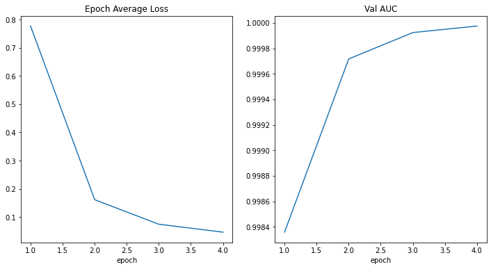
テストデータセット上でモデルを評価する
訓練と検証の後、検証テスト上のベストモデルを既に得ています。モデルをテストデータセット上でそれが堅牢で over fitting していないかを確認するために評価する必要があります。分類レポートを生成するためにこれらの予測を使用します。
model.load_state_dict(torch.load(
    os.path.join(root_dir, "best_metric_model.pth")))
model.eval()
y_true = []
y_pred = []
with torch.no_grad():
    for test_data in test_loader:
        test_images, test_labels = (
            test_data[0].to(device),
            test_data[1].to(device),
        )
        pred = model(test_images).argmax(dim=1)
        for i in range(len(pred)):
            y_true.append(test_labels[i].item())
            y_pred.append(pred[i].item())
print(classification_report( y_true, y_pred, target_names=class_names, digits=4))Note: you may need to restart the kernel to use updated packages. precision recall f1-score support AbdomenCT 0.9816 0.9917 0.9867 969 BreastMRI 0.9968 0.9831 0.9899 944 CXR 0.9979 0.9928 0.9954 973 ChestCT 0.9938 0.9990 0.9964 959 Hand 0.9934 0.9934 0.9934 1055 HeadCT 0.9960 0.9990 0.9975 985 accuracy 0.9932 5885 macro avg 0.9932 0.9932 0.9932 5885 weighted avg 0.9932 0.9932 0.9932 5885データディレクトリのクリーンアップ
一時ディレクトリが使用された場合ディレクトリを削除します。
if directory is None:
    shutil.rmtree(root_dir)
以上
MONAI 0.7 : モジュール概要 (1) 医用画像データI/O, 前処理と増強
MONAI 0.7 : モジュール概要 (1) 医用画像データI/O, 前処理と増強 (翻訳/解説)
翻訳 : (株)クラスキャット セールスインフォメーション
作成日時 : 10/05/2021 (0.7.0)
* 本ページは、MONAI の以下のドキュメントを翻訳した上で適宜、補足説明したものです:
* サンプルコードの動作確認はしておりますが、必要な場合には適宜、追加改変しています。
* ご自由にリンクを張って頂いてかまいませんが、sales-info@classcat.com までご一報いただけると嬉しいです。
- 人工知能研究開発支援
- 人工知能研修サービス(経営者層向けオンサイト研修)
- テクニカルコンサルティングサービス
- 実証実験(プロトタイプ構築)
- アプリケーションへの実装
- 人工知能研修サービス
- PoC(概念実証)を失敗させないための支援
- テレワーク & オンライン授業を支援
- お住まいの地域に関係なく Web ブラウザからご参加頂けます。事前登録 が必要ですのでご注意ください。
- ウェビナー運用には弊社製品「ClassCat® Webinar」を利用しています。
◆ お問合せ : 本件に関するお問い合わせ先は下記までお願いいたします。
| 株式会社クラスキャット セールス・マーケティング本部 セールス・インフォメーション |
| E-Mail:sales-info@classcat.com ; WebSite: https://www.classcat.com/ ; Facebook |
MONAI 0.7 : モジュール概要 (1) 医用画像データI/O, 前処理と増強
MONAI は医用画像解析における深層学習を様々な粒度でサポートすることを目的としています。この図は end-to-end ワークフローの典型的な例を示します :
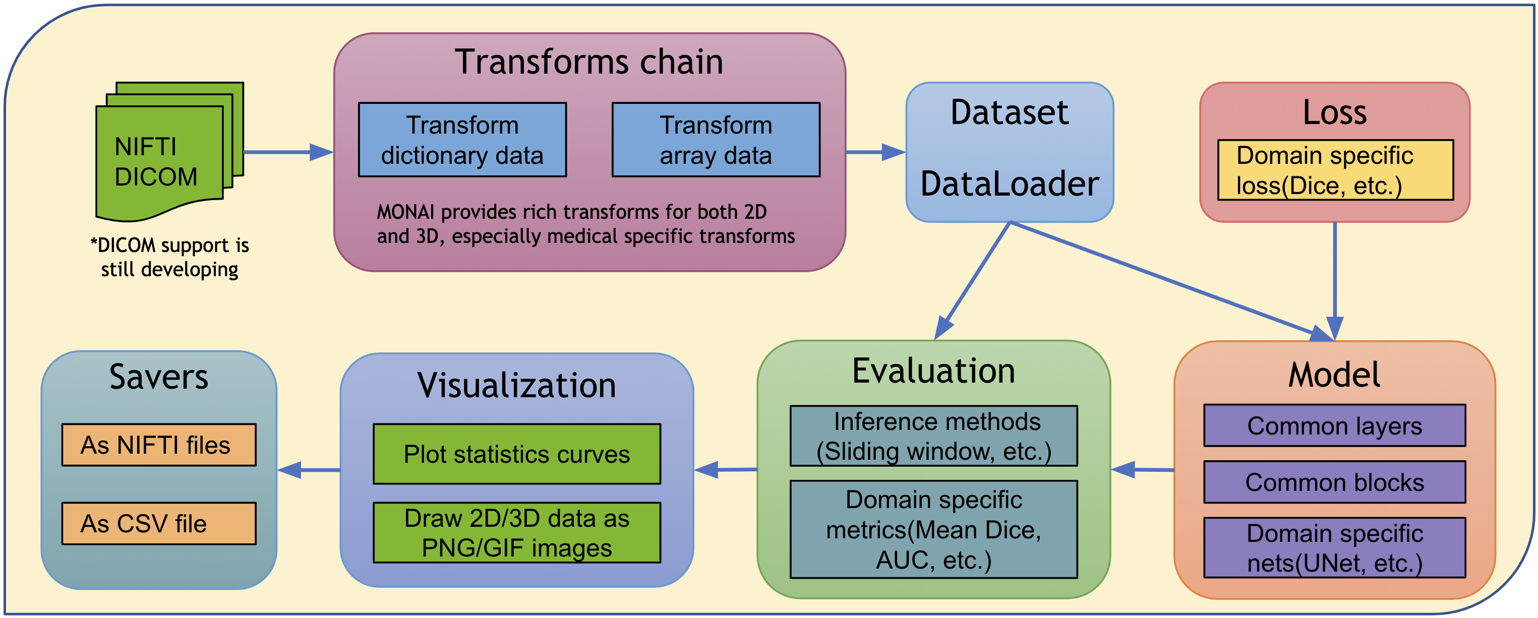
MONAI アーキテクチャ
MONAI の設計原理は様々な専門知識を持つユーザのために柔軟で軽量な API を提供することです。
- 総てのコアコンポーネントは独立したモジュールで、これらは任意の既存の PyTorch プログラムに容易に統合できます。
- ユーザは、研究実験のための堅固な訓練や評価プログラムを素早くセットアップするために MONAI のワークフローを活用できます。
- 主要な機能を実演するために豊富なサンプルとデモが提供されます。
- COVID-19 画像解析、モデル並列等を含む、最新の研究課題のための最先端技術に基づいて研究者が実装を提供しています。
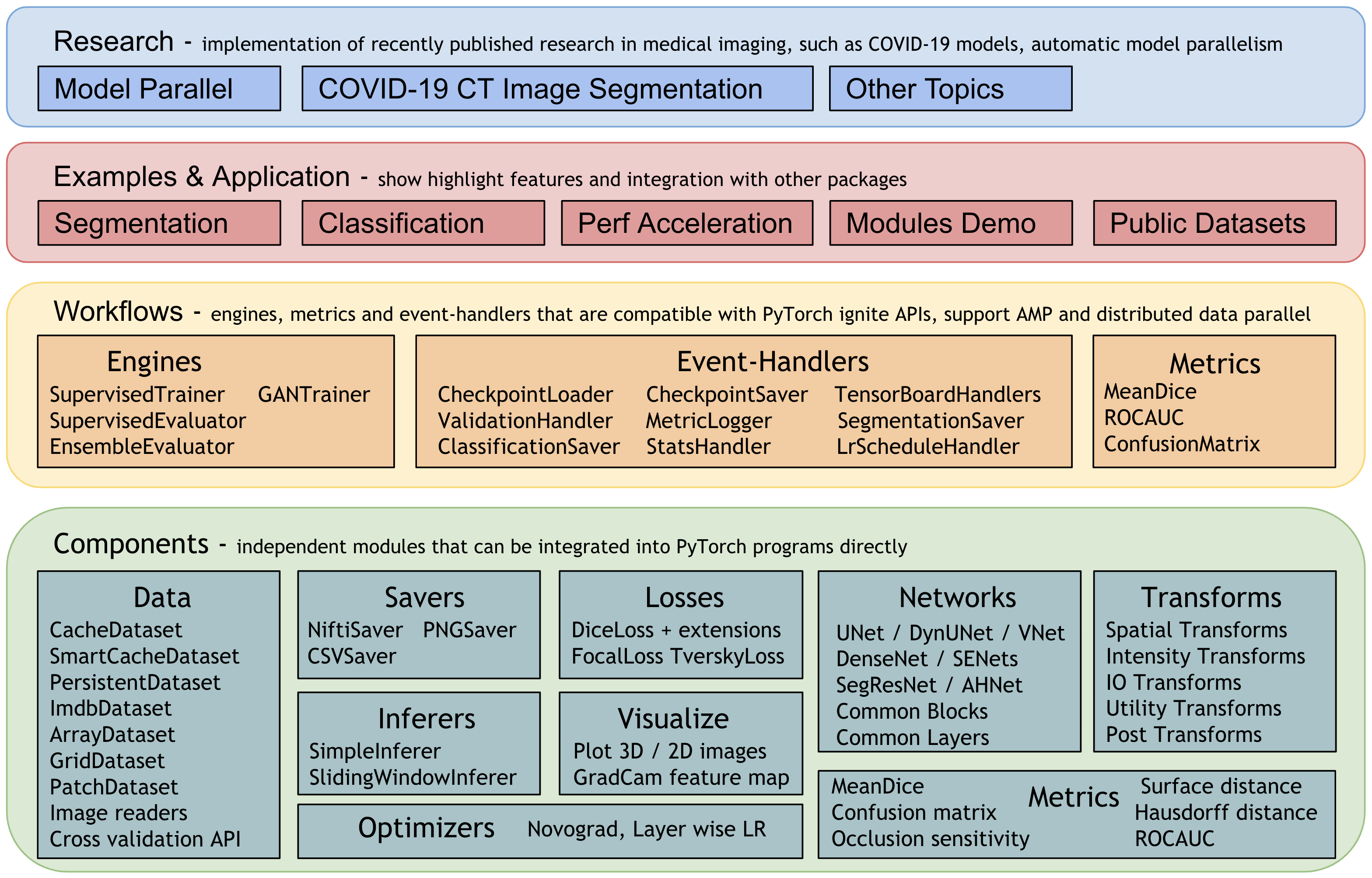
全体的なアーキテクチャとモジュールは次の図で示されます :
医用画像データ I/O、(前) 処理と増強
医用画像は I/O、前処理と増強のための高度に特化された方法を必要とします。医用画像は豊富なメタ情報を持つ特別な形式にあることが多く、データボリュームは高次元であることが多いです。これれは注意深く設計された操作手続きを必要とします。MONAI の医用画像フォーカスは強力で柔軟な画像変換により可能になります、これは使い勝手の良い、再現性のある、最適化された医療データ前処理パイプラインを容易にします。
1. 辞書と配列形式データの両方をサポートする変換
- (torchvision のような) 広く使用されているコンピュータビジョン・パッケージは空間的に 2D な配列画像処理にフォーカスしています。MONAI は空間的に 2D と 2D の両方のためによりドメイン固有な変換を提供し、そして柔軟な変換 “compose” 機能を保持しています。
- 医用画像前処理は追加の極め細かいシステムパラメータを必要とすることが多いので、MONAI は python 辞書にカプセル化された入力データのための変換を提供します。ユーザは複雑な変換を構成するために想定されるデータフィールドに対応するキーとシステムパラメータを指定できます。
6 つのカテゴリー内の変換の豊富なセットがあります : Crop & Pad, 強度, IO, 後処理, Spatial とユティリティです。詳細は、MONAI の変換の総て にアクセスしてください。
殆ど総ての変換は入力データがチャネル first の shape 形式を持つことを想定しています : [Channel dim, spatial dim 1, spatial dim 2, …] です。柔軟な ベース API がまた提供されます。monai.transforms モジュールは簡単に拡張可能です。
2. 医療に特化した変換
MONAI は包括的な医療に特化した変換を提供することを目的としています。これらが現在、例えば以下を含みます :
- LoadImage: 指定されたパスから医療固有の形式のファイルをロードする
- Spacing: 入力画像を指定された pixdim に再サンプリングする
- Orientation: 画像の方向を指定された axcodes に変更する
- RandGaussianNoise: 統計的なノイズを追加して画像強度を摂動を与える
- NormalizeIntensity: 平均と標準偏差に基づく強度正規化
- Affine: アフィン・パラメータに基づいて画像を変換する
- Rand2DElastic: ランダムな elastic 変形と 2D のアフィン
- Rand3DElastic: ランダムな elastic 変形と 3D のアフィン
2D 変換チュートリアル は幾つかの MONAI 医用画像特有の変換の詳細な使用方法を示します。
![]()
3. 変換は NumPy 配列と PyTorch テンソルの両方をサポートします (CPU or GPU accelerated)
MONAI v0.7 から変換で PyTorch テンソルベースの計算を導入しましたが、多くの変換は入力タイプと計算バックエンドとして NumPy 配列とテンソルを既にサポートしています。総ての変換のサポートされているバックエンドを取得するには、次を実行してください : python monai/transforms/utils.py.
変換を高速化するためには、一般的なアプローチは GPU 並列計算を利用することです。ユーザは最初に ToTensor または EnsureType 変換により入力データを GPU テンソルに変換し、それから続く変換を PyTorch テンソル API に基づいて GPU 上で実行できます。GPU 変換チュートリアルは Spleen 高速訓練チュートリアル で利用可能です。
4. 融合した空間変換
医用画像ボリュームは (多次元配列にあるので) 通常は大規模ですので、前処理パフォーマンスは全体的なパイプライン速度に影響します。MONAI は融合した空間操作を実行するアフィン変換を提供します。
例えば :
# create an Affine transform
affine = Affine(
    rotate_params=np.pi/4,
    scale_params=(1.2, 1.2),
    translate_params=(200, 40),
    padding_mode='zeros',
)
# convert the image using bilinear interpolation
new_img = affine(image, spatial_size=(300, 400), mode='bilinear')
実験とテスト結果は 融合した変換テスト で利用可能です。
現在、総ての幾何学的画像変換 (Spacing, ズーム, 回転, リサイズ 等) は PyTorch ネイティブ・インターフェイスに基づいて設計されています。そのためそれらの総ては高性能のための GPU テンソル演算を通して GPU 高速化をサポートしています。
幾何学的変換チュートリアル は 3D 医用画像でアフィン変換の使用方法を示します。
5. ポジティブ/ネガティブ比率に基づいてランダムにクロップ
医用画像データボリュームは GPU メモリに収まらないほど大きい場合があります。広く使用されているアプローチは、訓練の間は小さいデータサンプルをランダムにドローして推論のために「スライディング・ウィンドウ」ルーチンを実行することです。MONAI は現在、パッチベースの訓練プロセスを安定化させるのに役立つ可能性のある、クラス・バランスの取れた固定比率サンプリングを含む一般的なランダム・サンプリング・ストラテジーを提供しています。典型的な例は 脾臓 3D セグメンテーション・チュートリアル で、これは RandCropByPosNegLabel 変換とともにクラス・バランスのとれたサンプリングを実現しています。
6. 再現性のための決定論的訓練
決定論的訓練のサポートは深層学習研究、特に医療分野では必要で重要です。ユーザは MONAI の総てのランダム変換にランダムシードをローカルで簡単に設定できてユーザのプログラムの他の非決定論的モジュールに影響を与えません。
例えば :
# define a transform chain for pre-processing
train_transforms = monai.transforms.Compose([
    LoadImaged(keys=['image', 'label']),
    RandRotate90d(keys=['image', 'label'], prob=0.2, spatial_axes=[0, 2]),
    ... ...
])
# set determinism for reproducibility
train_transforms.set_random_state(seed=0)
ユーザはまた訓練プログラムの最初に決定論的 (動作) を有効/無効にできます :
monai.utils.set_determinism(seed=0, additional_settings=None)
7. マルチ変換チェイン
同じデータに様々な変換を適用して結果を連結するために、MONAI は、データ辞書の指定された項目のコピーを作成する CopyItems 変換と想定される次元の指定項目を組み合わせるために ConcatItems 変換を提供し、そしてまたメモリを節約するために不要な項目を削除するための DeleteItems 変換も提供します。
典型的な使用方法は同じ画像の強度を異なる範囲にスケールして結果を一緒に連結します。
![]()
8. DataStats で変換をデバッグする
変換が “compose” 関数と組み合わされるとき、特定の変換の出力を追跡することは容易ではありません。合成された変換のエラーをデバッグするのを手助けするために、MONAI は、データ shape, 値範囲, データ値, 追加情報等の中間的なデータ特性を表示するために DataStats のようなユティリティ変換を提供しています。それは自己充足的な変換で任意の変換チェインに統合できます。
9. モデル出力のための後処理変換
MONAI はまたモデル出力を処理するための後処理変換も提供しています。現在、変換は以下を含みます :
- 活性化層の追加 (Sigmoid, Softmax, etc.)。
- 下図 (b) のように、離散値 (Argmax, One-Hot, Threshold 値等) に変換します。
- マルチチャネル・データを複数のシングル・チャネルに分割する。
- 下図 (c) のように、接続コンポーネント分析に基づいてセグメンテーション・ノイズを除去する。
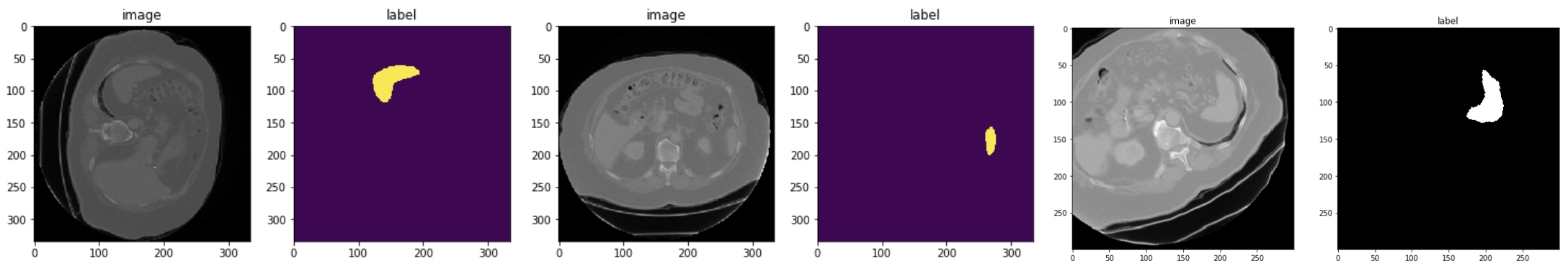
- 下図 (d) と (e) のように、セグメンテーション結果の輪郭を抽出します、これは元の画像へのマップに使用できてモデルを評価できます。
モデル出力のバッチデータを切り離し (= decollate) 後処理変換を適用した後では、メトリックを計算し、モデル出力をファイルにセーブし、あるいは TensorBoard でデータを可視化することは容易になります。後処理変換チュートリアル は後処理のための幾つかの主要な変換を使用するサンプルを示しています。
![]()
10. サードパーティの変換の統合
MONAI 変換の設計はコードの可読性と使い易さを重視しています。それは配列データや辞書ベースのデータのために動作します。MONAI はまた 3rd パーティの変換の異なるデータ形式に対応するためにアダプタ・ツールも提供しています。データ shape やタイプを変換するために ToTensor, ToNumpy, SqueezeDim のようなユティリティ変換も提供されます。従って、ITK, BatchGenerator, TorchIO と Rising を含む外部パッケージから変換をシームレスに統合することにより変換チェインを強化することは簡単です。
詳細は、チュートリアル: integrate 3rd party transforms into MONAI program を確認してください。
デジタル病理 (= pathology) 訓練では、画像のロードの膨大な負荷のために、CPU は画像のロードに先取りされてデータの前処理が追いつきません。これはパイプラインが IO に束縛されることを引き起こし GPU の使用率低下という結果になります。このボトルネックを解消するため、cuCIM は (私達がデジタル病理パイプラインで使用している) 幾つかの一般的な変換の最適化バージョンを実装しました。これらの変換は GPU 上でネイティブに実行されて CuPy 配列上動作します。MONAI は cuCIM ライブラリを統合するために CuCIM と RandCuCIM アダプタを提供しています。例えば :
RandCuCIM(name="color_jitter", brightness=64.0 / 255.0, contrast=0.75, saturation=0.25, hue=0.04)
CuCIM(name="scale_intensity_range", a_min=0.0, a_max=255.0, b_min=-1.0, b_max=1.0)
それは転移検出モデルの病理学の訓練で大幅なスピードアップを示しました。
11. 医用画像形式のための IO ファクトリー
多くのポピュラーな画像形式が医療ドメインに存在し、それらは豊富なメタデータ情報を持ち非常に異なります。同じパイプラインで異なる医用画像形式を簡単に処理するため、MONAI は LoadImage 変換を提供します、これはサポートされるサフィックスに基づいて以下の優先順位で画像リーダーを自動的に選択できます :
- このローダを呼び出すとき実行時にユーザに指定されたリーダー。
- 登録されたリーダー、リストの最新のものから最初のものへ。
- デフォルトのリーダ : (nii, nii.gz -> NibabelReader), (png, jpg, bmp -> PILReader), (npz, npy -> NumpyReader), (others -> ITKReader)。
ImageReader API は非常に簡単で、ユーザはカスタマイズされた画像リーダーのためにそれを簡単に拡張できます。
これらの事前定義された画像リーダーにより、MONAI は次の形式で画像をロードできます : NIfTI, DICOM, PNG, JPG, BMP, NPY/NPZ, 等々。
12. 変換データを NIfTI または PNG ファイルにセーブする
画像をファイルに変換したり、変換チェインをデバッグするため、MONAI は SaveImage 変換を提供しています。結果をセーブするためユーザはこの変換を変換チェインに注入できます。
13. チャネル first データ shape を自動的に確実にする
医用画像は様々な shape 形式を持ちます。それらはチャネル last、チャネル first あるいはノーチャネルでさえある可能性があります。例えば、幾つかのノーチャネル画像をロードしてそれらをチャネル first データとしてスタックすることを望むかもしれません。ユーザ体験を改善するため、MONAI はメタ情報に従ってデータ shape を自動的に検出してそれを一貫してチャネル first 形式に変換する EnsureChannelFirst 変換を提供しました。
14. 空間的変換とテスト時増強を反転する
深層学習ワークフローでは前に適用した空間的変換 (リサイズ, 反転, 回転, ズーム, クロップ, pad 等) を反転する (= inverse) ことが望ましい場合があります、例えば、正規化されたデータ空間で画像データを処理した後で元の画像空間に戻すためです。多くの空間的変換が 0.5 から反転演算で強化されています。モデル推論チュートリアル が基本的なサンプルを示しています。
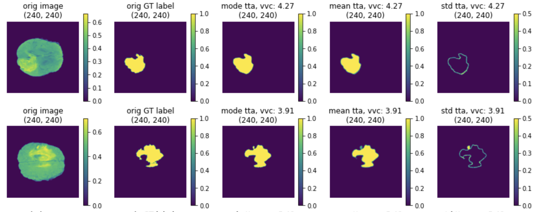
パイプラインがランダムな変換を含む場合、ユーザは出力上でこれらの変換が持つ効果を観察することを望むかもしれません。典型的なアプローチは、異なるランダムな具現化で複数回変換を通して同じ入力を渡すことです。そして総ての結果を共通の空間に移すために反転変換を使用して、メトリクスを計算します。MONAI はこの機能のために TestTimeAugmentation を提供しました、これはデフォルトで 最頻値, 平均値, 標準偏差と volume 変動係数を計算します。
Invert transforms and TTA チュートリアル は使用サンプルとともに API について詳細を紹介しています。
(1) 最後のカラムはモデル出力の反転されたデータです :
![]()
(2) 最頻値, 平均と標準偏差の TTA 結果 :
以上
MONAI 0.7 : PyTorch ユーザのための MONAI
MONAI 0.7 : PyTorch ユーザのための MONAI (翻訳/解説)
翻訳 : (株)クラスキャット セールスインフォメーション
作成日時 : 10/05/2021 (0.7.0)
* 本ページは、MONAI の以下のドキュメントを翻訳した上で適宜、補足説明したものです:
* サンプルコードの動作確認はしておりますが、必要な場合には適宜、追加改変しています。
* ご自由にリンクを張って頂いてかまいませんが、sales-info@classcat.com までご一報いただけると嬉しいです。
- 人工知能研究開発支援
- 人工知能研修サービス(経営者層向けオンサイト研修)
- テクニカルコンサルティングサービス
- 実証実験(プロトタイプ構築)
- アプリケーションへの実装
- 人工知能研修サービス
- PoC(概念実証)を失敗させないための支援
- テレワーク & オンライン授業を支援
- お住まいの地域に関係なく Web ブラウザからご参加頂けます。事前登録 が必要ですのでご注意ください。
- ウェビナー運用には弊社製品「ClassCat® Webinar」を利用しています。
◆ お問合せ : 本件に関するお問い合わせ先は下記までお願いいたします。
| 株式会社クラスキャット セールス・マーケティング本部 セールス・インフォメーション |
| E-Mail:sales-info@classcat.com ; WebSite: https://www.classcat.com/ ; Facebook |
MONAI 0.7 : PyTorch ユーザのための MONAI
このチュートリアルは MONAI API を簡単に紹介してその柔軟性と使い易さにハイライトを当てます。それは PyTorch の基本的な理解を前提とし、MONAI がヘルスケア画像の深層学習のためにドメインに最適化された機能を提供する方法を示します。
パッケージのインストール
MONAI のコア機能は Python (3.6+) で書かれていて Numpy (1.17+) and Pytorch (1.4+) にのみ依存しています。
このセクションは MONAI の最新版をインストールしてインストールを検証します。
# install the latest weekly preview version of MONAI
%pip install -q "monai-weekly[tqdm, nibabel, gdown, ignite]"
     |████████████████████████████████| 652 kB 11.0 MB/s
     |████████████████████████████████| 221 kB 52.5 MB/s
import warnings
warnings.filterwarnings("ignore")  # remove some scikit-image warnings

import monai
monai.config.print_config()
MONAI version: 0.7.dev2138
Numpy version: 1.19.5
Pytorch version: 1.9.0+cu102
MONAI flags: HAS_EXT = False, USE_COMPILED = False
MONAI rev id: bfc42f02d3bbbc1bfa36abbc71df8a6ca863bd76

Optional dependencies:
Pytorch Ignite version: 0.4.5
Nibabel version: 3.0.2
scikit-image version: 0.16.2
Pillow version: 7.1.2
Tensorboard version: 2.6.0
gdown version: 3.6.4
TorchVision version: 0.10.0+cu102
tqdm version: 4.62.2
lmdb version: 0.99
psutil version: 5.4.8
pandas version: 1.1.5
einops version: NOT INSTALLED or UNKNOWN VERSION.
transformers version: NOT INSTALLED or UNKNOWN VERSION.

For details about installing the optional dependencies, please visit:
    https://docs.monai.io/en/latest/installation.html#installing-the-recommended-dependencies
数行のコードでパブリックな医療画像データセットへアクセス
公開されているベンチマークの使用はオープンで再現性のある研究のために重要です。MONAI は良く知られた公開データセットへの素早いアクセスを提供することを目的としています。このセクションは医療セグメンテーション・デカスロン (= Medical Segmentation Decathlon ) のデータセットから始めます。
DecathlonDataset オブジェクトは torch.data.utils.Dataset の薄いラッパーです。それは __getitem__ と __len__ を実装していて、PyTorch の組込みデータローダ torch.data.utils.DataLoader と完全に互換です。
PyTorch データセット API と比較して、DecathlonDataset は以下の追加機能を持ちます :
- 自動的なデータのダウンロードと解凍
- データと前処理の中間結果のキャッシング
- 訓練、検証とテストのランダムな分割
from monai.apps import DecathlonDataset

dataset = DecathlonDataset(root_dir="./", task="Task05_Prostate", section="training", transform=None, download=True)
print(f"\nnumber of subjects: {len(dataset)}.\nThe first element in the dataset is {dataset[0]}.")
Task05_Prostate.tar: 229MB [00:15, 15.8MB/s]
Downloaded: ./Task05_Prostate.tar
Verified 'Task05_Prostate.tar', md5: 35138f08b1efaef89d7424d2bcc928db.
Writing into directory: ./.
Loading dataset: 100%|██████████| 26/26 [00:00<00:00, 107018.55it/s]
number of subjects: 26.
The first element in the dataset is {'image': 'Task05_Prostate/imagesTr/prostate_46.nii.gz', 'label': 'Task05_Prostate/labelsTr/prostate_46.nii.gz'}.
コードセクションは公開レポジトリから "Task05_Prostate.tar" (download=True) をダウンロードして、それを解凍し、そしてアーカイブにより提供される JSON ファイルを解析することにより DecathlonDataset を作成しました。
これは前立腺 (= prostate) 移行 (= transitional) ゾーンと周辺 (= peripheral) ゾーンの輪郭を描く (= delineate) ための 3 クラス・セグメンテーション・タスクです (背景, TZ, PZ クラス)。入力は 2 つの様式、つまり T2 と ADC MRI を持ちます。
len(dataset) と dataset[0] は、それぞれデータセットのサイズを問い合わせ、データセットの最初の要素を取り出します。データセットのためのどのような画像変換も指定していませんので、この iterable なデータセットの出力は画像とセグメンテーション・ファイル名の単なるペアです。
柔軟な画像データ変換
このセクションはファイル名をメモリ内のデータ配列に変換する MONAI 変換を導入します、これは深層学習モデルにより消費される準備ができます。前処理パイプラインのより多くのサンプルは tutorial レポジトリと開発者ガイドで利用可能です。ここでは画像前処理の主要な機能を簡単にカバーします。
配列 vs 辞書ベースの変換
配列変換は MONAI の基本的なビルディングブロックで、それは torchvision.transforms と同様な単純な callable です。2 つの違いがあります :
- MONAI 変換は医療画像特有の処理機能を実装しています。
- MONAI 変換は入力が numpy 配列、pytorch テンソルかテンソル like なオブジェクトであることを前提としています。
以下はローダー変換を開始します、これはファイル名文字列を実際の画像データに変換します。この変換への その他のオプションのドキュメント を参照してください。
from monai.transforms import LoadImage

loader = LoadImage(image_only=True)
img_array = loader("Task05_Prostate/imagesTr/prostate_02.nii.gz")
print(img_array.shape)
(320, 320, 24, 2)
辞書変換は配列バージョンのラッパーに過ぎません。配列ベースのものと比べて、同じ種類の演算やステートメントを複数のデータ入力に適用することが簡単です。
以下のセクションは画像とセグメンテーション・マスクのペアを読みます、変換が辞書のどの項目が処理されるべきかを知れるようにキーが指定される必要があることに注意してください。
from monai.transforms import LoadImageD

dict_loader = LoadImageD(keys=("image", "label"))
data_dict = dict_loader({"image": "Task05_Prostate/imagesTr/prostate_02.nii.gz",
                         "label": "Task05_Prostate/labelsTr/prostate_02.nii.gz"})
print(f"image shape: {data_dict['image'].shape}, \nlabel shape: {data_dict['label'].shape}")
image shape: (320, 320, 24, 2),
label shape: (320, 320, 24)
変換の構成
多くの場合、変換のチェインを構築して、前処理パラメータを調整して、高速な前処理パイプラインを作成することは有益です。monai.transforms.Compose はこれらのユースケースのために設計されています。
以下のコードは複数の前処理ステップを行なうために変換チェインを開始しています :
- Nifti 画像を (画像メタデータ情報と共に) ロードします
- 画像とラベルの両方をチャネル first にする (画像を reshape してラベルのためにチャネル次元を追加します)
- 画像とラベルを 1 mm 四方にする
- 画像とラベルの両方を "RAS" 座標系にあるようにする
- 画像強度をスケールする
- 画像とラベルを空間サイズ (64, 64, 32) mm にリサイズする
- 画像をランダムに回転とスケールしますが、出力サイズは (64, 64, 32) mm に保持します。
- 画像とラベルを torch テンソルに変換する
import numpy as np
from monai.transforms import \
    LoadImageD, EnsureChannelFirstD, AddChannelD, ScaleIntensityD, ToTensorD, Compose, \
    AsDiscreteD, SpacingD, OrientationD, ResizeD, RandAffineD
KEYS = ("image", "label")

xform = Compose([
    LoadImageD(KEYS),
    EnsureChannelFirstD("image"),
    AddChannelD("label"),
    SpacingD(KEYS, pixdim=(1., 1., 1.), mode=('bilinear', 'nearest')),
    OrientationD(KEYS, axcodes='RAS'),
    ScaleIntensityD(keys="image"),
    ResizeD(KEYS, (64, 64, 32), mode=('trilinear', 'nearest')),
    RandAffineD(KEYS, spatial_size=(-1, -1, -1),
                rotate_range=(0, 0, np.pi/2),
                scale_range=(0.1, 0.1),
                mode=('bilinear', 'nearest'),
                prob=1.0),
    ToTensorD(KEYS),
])

data_dict = xform({"image": "Task05_Prostate/imagesTr/prostate_02.nii.gz",
                   "label": "Task05_Prostate/labelsTr/prostate_02.nii.gz"})
print(data_dict["image"].shape, data_dict["label"].shape)
torch.Size([2, 64, 64, 32]) torch.Size([1, 64, 64, 32])
MONAI には有用な変換のセットがあり、今後更に増えます。詳細は https://docs.monai.io/en/latest/transforms.html を見てください。
データセット、変換とデータローダ
私達が持っているものをまとめると :
- Dataset : torch.utils.data.Dataset の薄いラッパー
- Transform : callable、Compose により作成される変換チェインの一部です。
- データセットへの変換のセットはデータロードと前処理パイプラインを可能にします。
パイプラインは pytorch ネイティブのデータローダと連携できて、これはマルチプロセスのサポートと柔軟なバッチサンプリング・スキームを提供します。
けれども、MONAI データローダ monai.data.DataLoader と連携することが推奨されます、これは pytorch ネイティブのラッパーです。MONAI データローダは以下の機能を主として追加します :
- マルチプロセスのコンテキストでランダム化された増強を正しく処理します。
- マルチサンプルデータのリストを個々の訓練サンプルに平坦化するためのカスタマイズされた collate 関数
import torch
from monai.data import DataLoader

# start a chain of transforms
xform = Compose([
    LoadImageD(KEYS),
    EnsureChannelFirstD("image"),
    AddChannelD("label"),
    SpacingD(KEYS, pixdim=(1., 1., 1.), mode=('bilinear', 'nearest')),
    OrientationD(KEYS, axcodes='RAS'),
    ScaleIntensityD(keys="image"),
    ResizeD(KEYS, (64, 64, 32), mode=('trilinear', 'nearest')),
    RandAffineD(KEYS, spatial_size=(-1, -1, -1),
                rotate_range=(0, 0, np.pi/2),
                scale_range=(0.1, 0.1),
                mode=('bilinear', 'nearest'),
                prob=1.0),
    ToTensorD(KEYS),
])
# start a dataset
dataset = DecathlonDataset(root_dir="./", task="Task05_Prostate", section="training", transform=xform, download=True)

# start a pytorch dataloader
# data_loader = torch.utils.data.DataLoader(dataset, batch_size=1, shuffle=False, num_workers=1)
data_loader = DataLoader(dataset, batch_size=1, shuffle=True, num_workers=1)
Verified 'Task05_Prostate.tar', md5: 35138f08b1efaef89d7424d2bcc928db.
File exists: ./Task05_Prostate.tar, skipped downloading.
Non-empty folder exists in ./Task05_Prostate, skipped extracting.
Loading dataset: 100%|██████████| 26/26 [00:17<00:00,  1.51it/s]
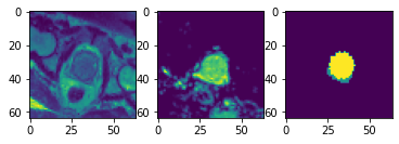
data_dict で何が起きているか覗いてみましょう (以下のセクションの再実行はデータセットからのランダムに増強されたサンプルを生成します) :
import matplotlib.pyplot as plt
import numpy as np

data_dict = next(iter(data_loader))
print(data_dict["image"].shape, data_dict["label"].shape, data_dict["image_meta_dict"]["filename_or_obj"])

plt.subplots(1, 3)
plt.subplot(1, 3, 1); plt.imshow(data_dict["image"][0, 0, ..., 16])
plt.subplot(1, 3, 2); plt.imshow(data_dict["image"][0, 1, ..., 16])
plt.subplot(1, 3, 3); plt.imshow(data_dict["label"][0, 0, ..., 16])
plt.show()

print(f"unique labels: {np.unique(data_dict['label'])}")
torch.Size([1, 2, 64, 64, 32]) torch.Size([1, 1, 64, 64, 32]) ['Task05_Prostate/imagesTr/prostate_42.nii.gz']
データローダは、深層学習モデルに対応できるように、画像とラベルの両方にバッチ次元を追加しました。
ラベルのために "nearest" 補完モードが使用されますので、変換中に一意のクラスの数が保持されます。
層、ブロック、ネットワークと損失関数
データ入力パイプラインを通り抜けました。適切に前処理されたデータは、2 つの様式の入力を使用して 3 クラス・セグメンテーション・タスクのための準備ができました。
このセクションは UNet モデル、そして損失関数と optimzer を作成します。これら総てのモジュールは (torch.nn.Module のような) PyTorch インターフェイスの直接的な使用か拡張です。それらは、コードが標準 PyTorch API に従うのであれば、任意のカスタマイズされた Python コードで置き換え可能です。
MONAI のモジュールは医療画像解析のために拡張モジュールを提供することに焦点を当てています :
- 柔軟性とコード可読性の両者を目的とした参照ネットワークの実装
- 1D, 2D と 3D ネットワークと互換な事前定義された層とブロック
- ドメイン固有の損失関数
from monai.networks.nets import UNet
from monai.networks.layers import Norm
from monai.losses import DiceLoss

device = torch.device('cuda:0')
net = UNet(dimensions=3, in_channels=2, out_channels=3, channels=(16, 32, 64, 128, 256),
           strides=(2, 2, 2, 2), num_res_units=2, norm=Norm.BATCH).to(device)
loss = DiceLoss(to_onehot_y=True, softmax=True)
opt = torch.optim.Adam(net.parameters(), 1e-2)
`UNet` は `dimensions` パラメータで定義されます。それは Conv1d, Conv2d と Conv3d のような、pytorch API の空間次元の数を指定します。同じ実装で、1D, 2D, 3D とマルチモーダル訓練のために容易に構成できます。
`torch.nn.Module` の拡張としての `UNet` は特定の方法で体系化された MONAI ブロックと層のセットです。ブロックと層は、"Conv. + Feature Norm. + Activation" のような一般に使用される組合せのように、再利用可能なサブモジュールとして設計されています。
スライディング・ウィンドウ推論
この一般に使用されるモジュールについて、MONAI は単純な PyTorch ベースの実装を提供します、これはウィンドウサイズと入力モデル (これは torch.nn.Module 実装であり得ます) の仕様だけを必要とします。
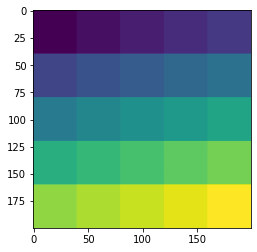
以下のデモは、総ての空間位置を通して実行される (40, 40) 空間サイズ・ウィンドウ を集約することにより、(1, 1, 200, 200) の入力画像上のスライディング・ウィンドウ推論の toy を示します。
roi_size, sw_batch_size と overlap パラメータをそれらのスライディング・ウィンドウ出力上のインパクトを見るために変更することができます。
from monai.inferers import SlidingWindowInferer

class ToyModel:
    # A simple model generates the output by adding an integer `pred` to input.
    # each call of this instance increases the integer by 1.
    pred = 0
    def __call__(self, input):
        self.pred = self.pred + 1
        input = input + self.pred
        return input

infer = SlidingWindowInferer(roi_size=(40, 40), sw_batch_size=1, overlap=0)
input_tensor = torch.zeros(1, 1, 200, 200)
output_tensor = infer(input_tensor, ToyModel())
plt.imshow(output_tensor[0, 0]); plt.show()
訓練ワークフローの開始 (エポック毎に検証)
入力パイプライン、ネットワーク・アーキテクチャ、損失関数は総て既存の pytorch ベースのワークフローと互換です。様々なユースケースについてはチュートリアルを参照してください : https://github.com/Project-MONAI/tutorials
ここで PyTorch-Ignite ベースで MONAI により構築された、ワークフロー・ユティリティにハイライトを当てたいです。主要な目標は、比較的標準的な訓練ワークフローを構築する際にユーザの労力を軽減することです。
import ignite
print(ignite.__version__)
0.4.5
以下のコマンドは SupervisedTrainer インスタンスを起動します。PyTorch ignite の機能の拡張として、それは前に言及した総ての要素を結合します。trainer.run() の呼び出しは 2 エポックの間ネットワークを訓練して、総てのエポックの最後に訓練データに基づいて MeadDice メトリックを計算します。
key_train_metric はモデルの品質向上の進捗を追跡するために使用されます。
早期停止と学習率スケジューリングを行なうために追加のハンドラが設定可能です。StatsHandler は診断情報を stdout にプリントするために各訓練反復でトリガーされます。これらはユーザ指定の頻度で詳細な訓練ログを生成するように構成できます。イベント処理システムの詳細は、ドキュメント https://docs.monai.io/en/latest/handlers.html を参照してください。
注目すべき点は、これらの機能は通常の訓練と検証パイプラインの高速なプロトタイピングを容易にすることです。ユーザは前のセクションで述べたモジュールを利用して、独自のパイプラインを構築することを常に選択できます。
from monai.engines import SupervisedTrainer
from monai.inferers import SlidingWindowInferer
from monai.handlers import StatsHandler, MeanDice, from_engine
from monai.transforms import AsDiscreteD

import sys
import logging
logging.basicConfig(stream=sys.stdout, level=logging.INFO)

trainer = SupervisedTrainer(
    device=device,
    max_epochs=2,
    train_data_loader=data_loader,
    network=net,
    optimizer=opt,
    loss_function=loss,
    inferer=SlidingWindowInferer((32, 32, -1), sw_batch_size=2),
    postprocessing=AsDiscreteD(keys=["pred", "label"], argmax=(True, False), to_onehot=True, n_classes=3),
    key_train_metric={"train_meandice": MeanDice(output_transform=from_engine(["pred", "label"]))},
    train_handlers=StatsHandler(tag_name="train_loss", output_transform=from_engine(["loss"], first=True)),
)
trainer.run()
INFO:ignite.engine.engine.SupervisedTrainer:Engine run resuming from iteration 0, epoch 0 until 2 epochs
INFO:ignite.engine.engine.SupervisedTrainer:Epoch: 1/2, Iter: 1/26 -- train_loss: 0.8139
INFO:ignite.engine.engine.SupervisedTrainer:Epoch: 1/2, Iter: 2/26 -- train_loss: 0.7707
INFO:ignite.engine.engine.SupervisedTrainer:Epoch: 1/2, Iter: 3/26 -- train_loss: 0.6901
INFO:ignite.engine.engine.SupervisedTrainer:Epoch: 1/2, Iter: 4/26 -- train_loss: 0.6979
INFO:ignite.engine.engine.SupervisedTrainer:Epoch: 1/2, Iter: 5/26 -- train_loss: 0.7192
INFO:ignite.engine.engine.SupervisedTrainer:Epoch: 1/2, Iter: 6/26 -- train_loss: 0.6859
INFO:ignite.engine.engine.SupervisedTrainer:Epoch: 1/2, Iter: 7/26 -- train_loss: 0.6445
INFO:ignite.engine.engine.SupervisedTrainer:Epoch: 1/2, Iter: 8/26 -- train_loss: 0.6273
INFO:ignite.engine.engine.SupervisedTrainer:Epoch: 1/2, Iter: 9/26 -- train_loss: 0.6346
INFO:ignite.engine.engine.SupervisedTrainer:Epoch: 1/2, Iter: 10/26 -- train_loss: 0.6078
INFO:ignite.engine.engine.SupervisedTrainer:Epoch: 1/2, Iter: 11/26 -- train_loss: 0.5424
INFO:ignite.engine.engine.SupervisedTrainer:Epoch: 1/2, Iter: 12/26 -- train_loss: 0.5851
INFO:ignite.engine.engine.SupervisedTrainer:Epoch: 1/2, Iter: 13/26 -- train_loss: 0.5647
INFO:ignite.engine.engine.SupervisedTrainer:Epoch: 1/2, Iter: 14/26 -- train_loss: 0.5551
INFO:ignite.engine.engine.SupervisedTrainer:Epoch: 1/2, Iter: 15/26 -- train_loss: 0.5925
INFO:ignite.engine.engine.SupervisedTrainer:Epoch: 1/2, Iter: 16/26 -- train_loss: 0.5389
INFO:ignite.engine.engine.SupervisedTrainer:Epoch: 1/2, Iter: 17/26 -- train_loss: 0.5662
INFO:ignite.engine.engine.SupervisedTrainer:Epoch: 1/2, Iter: 18/26 -- train_loss: 0.6309
INFO:ignite.engine.engine.SupervisedTrainer:Epoch: 1/2, Iter: 19/26 -- train_loss: 0.6168
INFO:ignite.engine.engine.SupervisedTrainer:Epoch: 1/2, Iter: 20/26 -- train_loss: 0.5556
INFO:ignite.engine.engine.SupervisedTrainer:Epoch: 1/2, Iter: 21/26 -- train_loss: 0.5243
INFO:ignite.engine.engine.SupervisedTrainer:Epoch: 1/2, Iter: 22/26 -- train_loss: 0.5801
INFO:ignite.engine.engine.SupervisedTrainer:Epoch: 1/2, Iter: 23/26 -- train_loss: 0.5132
INFO:ignite.engine.engine.SupervisedTrainer:Epoch: 1/2, Iter: 24/26 -- train_loss: 0.4951
INFO:ignite.engine.engine.SupervisedTrainer:Epoch: 1/2, Iter: 25/26 -- train_loss: 0.4870
INFO:ignite.engine.engine.SupervisedTrainer:Epoch: 1/2, Iter: 26/26 -- train_loss: 0.5108
INFO:ignite.engine.engine.SupervisedTrainer:Got new best metric of train_meandice: 0.4181462824344635
INFO:ignite.engine.engine.SupervisedTrainer:Epoch[1] Metrics -- train_meandice: 0.4181
INFO:ignite.engine.engine.SupervisedTrainer:Key metric: train_meandice best value: 0.4181462824344635 at epoch: 1
INFO:ignite.engine.engine.SupervisedTrainer:Epoch[1] Complete. Time taken: 00:00:08
INFO:ignite.engine.engine.SupervisedTrainer:Epoch: 2/2, Iter: 1/26 -- train_loss: 0.5620
INFO:ignite.engine.engine.SupervisedTrainer:Epoch: 2/2, Iter: 2/26 -- train_loss: 0.5373
INFO:ignite.engine.engine.SupervisedTrainer:Epoch: 2/2, Iter: 3/26 -- train_loss: 0.4764
INFO:ignite.engine.engine.SupervisedTrainer:Epoch: 2/2, Iter: 4/26 -- train_loss: 0.5111
INFO:ignite.engine.engine.SupervisedTrainer:Epoch: 2/2, Iter: 5/26 -- train_loss: 0.5922
INFO:ignite.engine.engine.SupervisedTrainer:Epoch: 2/2, Iter: 6/26 -- train_loss: 0.5519
INFO:ignite.engine.engine.SupervisedTrainer:Epoch: 2/2, Iter: 7/26 -- train_loss: 0.6246
INFO:ignite.engine.engine.SupervisedTrainer:Epoch: 2/2, Iter: 8/26 -- train_loss: 0.4363
INFO:ignite.engine.engine.SupervisedTrainer:Epoch: 2/2, Iter: 9/26 -- train_loss: 0.5052
INFO:ignite.engine.engine.SupervisedTrainer:Epoch: 2/2, Iter: 10/26 -- train_loss: 0.5900
INFO:ignite.engine.engine.SupervisedTrainer:Epoch: 2/2, Iter: 11/26 -- train_loss: 0.5997
INFO:ignite.engine.engine.SupervisedTrainer:Epoch: 2/2, Iter: 12/26 -- train_loss: 0.4996
INFO:ignite.engine.engine.SupervisedTrainer:Epoch: 2/2, Iter: 13/26 -- train_loss: 0.4969
INFO:ignite.engine.engine.SupervisedTrainer:Epoch: 2/2, Iter: 14/26 -- train_loss: 0.5740
INFO:ignite.engine.engine.SupervisedTrainer:Epoch: 2/2, Iter: 15/26 -- train_loss: 0.5852
INFO:ignite.engine.engine.SupervisedTrainer:Epoch: 2/2, Iter: 16/26 -- train_loss: 0.5460
INFO:ignite.engine.engine.SupervisedTrainer:Epoch: 2/2, Iter: 17/26 -- train_loss: 0.5034
INFO:ignite.engine.engine.SupervisedTrainer:Epoch: 2/2, Iter: 18/26 -- train_loss: 0.5233
INFO:ignite.engine.engine.SupervisedTrainer:Epoch: 2/2, Iter: 19/26 -- train_loss: 0.5109
INFO:ignite.engine.engine.SupervisedTrainer:Epoch: 2/2, Iter: 20/26 -- train_loss: 0.4877
INFO:ignite.engine.engine.SupervisedTrainer:Epoch: 2/2, Iter: 21/26 -- train_loss: 0.5745
INFO:ignite.engine.engine.SupervisedTrainer:Epoch: 2/2, Iter: 22/26 -- train_loss: 0.5044
INFO:ignite.engine.engine.SupervisedTrainer:Epoch: 2/2, Iter: 23/26 -- train_loss: 0.4623
INFO:ignite.engine.engine.SupervisedTrainer:Epoch: 2/2, Iter: 24/26 -- train_loss: 0.4399
INFO:ignite.engine.engine.SupervisedTrainer:Epoch: 2/2, Iter: 25/26 -- train_loss: 0.4553
INFO:ignite.engine.engine.SupervisedTrainer:Epoch: 2/2, Iter: 26/26 -- train_loss: 0.5245
INFO:ignite.engine.engine.SupervisedTrainer:Got new best metric of train_meandice: 0.4688393473625183
INFO:ignite.engine.engine.SupervisedTrainer:Epoch[2] Metrics -- train_meandice: 0.4688
INFO:ignite.engine.engine.SupervisedTrainer:Key metric: train_meandice best value: 0.4688393473625183 at epoch: 2
INFO:ignite.engine.engine.SupervisedTrainer:Epoch[2] Complete. Time taken: 00:00:08
INFO:ignite.engine.engine.SupervisedTrainer:Engine run complete. Time taken: 00:00:16
決定論的訓練
決定論的訓練サポートは再現可能な研究のために重要です。MONAI は現在 2 つのメカニズムを提供しています :
- 総てのランダム変換のランダム状態を設定します。これはグローバルなランダム状態には影響しません。例えば :
# define a transform chain for pre-processing train_transforms = monai.transforms.Compose([ LoadNiftid(keys=['image', 'label']), RandRotate90d(keys=['image', 'label'], prob=0.2, spatial_axes=[0, 2]), ... ... ]) # set determinism for reproducibility train_transforms.set_random_state(seed=0) - 1行のコードでグローバルに python, numpy と pytorch のための決定論的訓練を有効にします、例えば :
monai.utils.set_determinism(seed=0, additional_settings=None)
まとめ
MONAI の主要なモジュールを通り抜けてきました。高度に柔軟な拡張とラッパーを作成することにより、MONAI は医療画像解析の観点から pytorch API を強化しています。
以下のような、この短いチュートリアルではカバーされなかったソフトウェア機能があります :
- 後処理変換
- 視覚化インターフェイス
- サードパーティの医療画像ツールキットからの組み込めるデータ変換
- 他の人気のある深層学習フレームワークを使用するワークフローの構築
- MONAI 研究
最新のマイルストーンのハイライトの詳細については、https://docs.monai.io/en/latest/highlights.html にアクセスしてください。
MONAI を深く理解するには、examples レポジトリは良い開始点です : https://github.com/Project-MONAI/tutorials
API ドキュメントについては、https://docs.monai.io にアクセスしてください。
以上
MONAI 0.7 : 概要 (README)
MONAI 0.7 : README (概要) (翻訳/解説)
翻訳 : (株)クラスキャット セールスインフォメーション
作成日時 : 10/03/2021 (0.7.0)
* 本ページは、MONAI の以下のドキュメントを翻訳した上で適宜、補足説明したものです:
* サンプルコードの動作確認はしておりますが、必要な場合には適宜、追加改変しています。
* ご自由にリンクを張って頂いてかまいませんが、sales-info@classcat.com までご一報いただけると嬉しいです。
- 人工知能研究開発支援
- 人工知能研修サービス(経営者層向けオンサイト研修)
- テクニカルコンサルティングサービス
- 実証実験(プロトタイプ構築)
- アプリケーションへの実装
- 人工知能研修サービス
- PoC(概念実証)を失敗させないための支援
- テレワーク & オンライン授業を支援
- お住まいの地域に関係なく Web ブラウザからご参加頂けます。事前登録 が必要ですのでご注意ください。
- ウェビナー運用には弊社製品「ClassCat® Webinar」を利用しています。
◆ お問合せ : 本件に関するお問い合わせ先は下記までお願いいたします。
| 株式会社クラスキャット セールス・マーケティング本部 セールス・インフォメーション |
| E-Mail:sales-info@classcat.com ; WebSite: https://www.classcat.com/ ; Facebook |
![]()
MONAI 0.7 : 概要 (README)
Medical Open Network for AI
MONAI は PyTorch エコシステムの一部で、ヘルスケア画像化における深層学習のための PyTorch ベース、オープンソースのフーレムワークです。その目標は :
- 共通基盤で協力して取り組める学術的、産業的そして臨床的な研究者のコミュニティを構築すること ;
- ヘルスケア画像化のための最先端な、end-to-end な訓練ワークフローを作成すること ;
- 深層学習モデルを作成して評価するために研究者に最適化され標準化された方法を提供すること。
機能
コードベースは現在活発な開発下にあります。現在のマイルストーン・リリースの テクニカル・ハイライト と What’s New を参照してください。
- 多次元医療画像データのための柔軟な前処理 ;
- 既存のワークフローとの簡単な統合のための構成的 & 可搬な API ;
- ネットワーク、損失、評価メトリクス等のためのドメイン固有実装 ;
- 様々なユーザ専門性のためのカスタマイズ可能なデザイン ;
- マルチ GPU データ並列サポート。
インストール
現在のリリース をインストールするには、単純に以下を実行します :
pip install monai
他のインストール方法 (デフォルト GitHub ブランチの使用、Docker の使用等) については、インストールガイド を参照してください。
Getting Started
MedNIST デモ と MONAI for PyTorch Users が Colab で利用可能です。
サンプルとノートブック・チュートリアルは Project-MONAI/tutorials にあります。
技術文書は docs.monai.io で利用可能です。
Contributing
MONAI への contribution (貢献) を行なうガイダンスについては、contributing ガイドライン を参照してください。
コミュニティ
Twitter @ProjectMONAI の会話に参加するか Slack チャネル に参加してください。
MONAI’s GitHub Discussions タブ で質問したり回答したりしてください。
リンク
- Website : https://monai.io/
- API ドキュメント : https://docs.monai.io
- Code: https://github.com/Project-MONAI/MONAI
- Project tracker: https://github.com/Project-MONAI/MONAI/projects
- Issue tracker: https://github.com/Project-MONAI/MONAI/issues
- Wiki : https://github.com/Project-MONAI/MONAI/wiki
- Test status: https://github.com/Project-MONAI/MONAI/actions
- PyPI package: https://pypi.org/project/monai/
- Weekly previews: https://pypi.org/project/monai-weekly/
- Docker Hub: https://hub.docker.com/r/projectmonai/monai
以上
pydicom 2.2 : ユーザガイド : Pixel データの操作
pydicom 2.2 : ユーザガイド : Pixel データの操作 (翻訳/解説)
翻訳 : (株)クラスキャット セールスインフォメーション
作成日時 : 09/27/2021 (v2.2.1)
* 本ページは、pydicom の以下のドキュメントを翻訳した上で適宜、補足説明したものです:
- User Guide : Working with Pixel Data
* サンプルコードの動作確認はしておりますが、必要な場合には適宜、追加改変しています。
* ご自由にリンクを張って頂いてかまいませんが、sales-info@classcat.com までご一報いただけると嬉しいです。
- 人工知能研究開発支援
- 人工知能研修サービス(経営者層向けオンサイト研修)
- テクニカルコンサルティングサービス
- 実証実験(プロトタイプ構築)
- アプリケーションへの実装
- 人工知能研修サービス
- PoC(概念実証)を失敗させないための支援
- テレワーク & オンライン授業を支援
- お住まいの地域に関係なく Web ブラウザからご参加頂けます。事前登録 が必要ですのでご注意ください。
- ウェビナー運用には弊社製品「ClassCat® Webinar」を利用しています。
◆ お問合せ : 本件に関するお問い合わせ先は下記までお願いいたします。
| 株式会社クラスキャット セールス・マーケティング本部 セールス・インフォメーション |
| E-Mail:sales-info@classcat.com ; WebSite: https://www.classcat.com/ ; Facebook |
pydicom 2.2 : ユーザガイド : Pixel データの操作
pydicom の pixel データを操作する方法。
イントロダクション
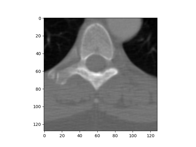
多くの DICOM SOP クラスはバルク pixel データを含みます、これは通常は 1 つ以上の画像フレームを表わすために使用されます (但し 他のデータ型 も可能です)。これらの SOP クラスでは pixel データは (殆ど) 常に (7FE0,0010) Pixel Data 要素に含まれます。これに対する唯一の例外は Parametric Map Storage です、これは代わりに (7FE0,0008) Float Pixel Data か (7FE0,0009) Double Float Pixel Data 要素にデータを含む場合があります。
Note : In the following the term pixel data will be used to refer to the bulk data from Pixel Data, Float Pixel Data and Double Float Pixel Data elements. While the examples use PixelData, FloatPixelData or DoubleFloatPixelData could also be used interchangeably provided the dataset contains the corresponding element.
デフォルトでは pydicom は pixel データをファイル内の raw バイトとして読み込みます :
from pydicom import dcmread
from pydicom.data import get_testdata_file
filename = get_testdata_file("MR_small.dcm")
ds = dcmread(filename)
ds.PixelData
b'\x89\x03\xfb\x03\xcb\x04\xeb\x04\xf9\x02\x94\x01\x7f\x02\x92\x038\x05a\x08g\x04%\x04=\x03\x1e\x02\x86\x01i\x01l\x01\x7f\x01\x8d\x01\x92\x01\x90\x01`\x01C\x011\x01,\x01;\x01Z\x016\x01\x8b\x01\xb7\x01\xcb\x01\xa6\x01?\x01i\x01\x83\x01\xb1\x01s\x010\x01+\x01\x10\x01\x13\x01x\x01J\x02\xfb\x02\x9f\x03\xa4\x04\xe2\x03\xc9\x02\x17\x02\x89\x01\xb5\x01\xa1\x01Q\x01\\\x01\r\x01\x17\x01!\x01)\x01\x18\x01\x11\x01\x03\x01.\x010\x01H\x01t\x02\x02\x03\x8b\x03\x8e\x04(\x04H\x02\x89\x01g\x02\x8c\x03\xff\x05\xcc\x07\xd7\x04\x81\x03}\x02\xc4\x01S\x01e\x01g\x01n\x01\x8e\x01\x88\x01s\x01C\x01+\x01=\x01D\x01e\x01L\x01@\x01[\x01x\x01\xb4\x01G\x01+\x01I\x01\x90\x01<\x01\x15\x01\x08\x01\x04\x01\x13\x01\x13\x01v\x01>\x02\xfe\x02s\x04\x80\x04\xed\x02\xfa\x01m\x01\x9f\x01\x92\x01o\x01 \x01\x08\x01\xf6\x00\xf5\x00\x03\x01\x19\x01\xfd\x00\xff\x00*\x01K\x01c\x01\xf2\x016\x02\xc2\x02S\x03~\x04%\x03\xc3\x01\xa0\x01p\x02\x94\x03\xef\x05T\x06\x15\x04\xc0\x02\x96\x02\x8d\x01K\x01O\x01b\x01z\x01\x9b\x01|\x01G\x01.\x01\x1b\x01H\x01\\\x01b\x01\\\x01I\x01R\x01X\x01\x84\x01\x1f\x01&\x01e\x01"\x01\x07\x01\n\x01\x03\x01\xfc\x00\x07\x01,\x01\x82\x01x\x02\xe4\x03\xa3\x04{\x03.\x02d\x01q\x01V\x01K\x01 \x01\xfb\x00\xff\x00\xeb\x00\xe0\x00\xfe\x00\x07\x01\xf7\x00\x18\x01\x1d\x01@\x01\xf4\x01\xd6\x01\x1a\x02\xab\x02L\x03:\x04\xc3\x02z\x01\xdb\x01\xf7\x021\x04*\x05\xe7\x03\x9a\x03\xfa\x02*\x02^\x01D\x01\x87\x01\xa3\x01\xab\x01t\x01^\x01A\x01\x1a\x01\x18\x01<\x011\x01&\x01B\x01\\\x01o\x016\x01\x1b\x01\x18\x01.\x01\x0b\x01\xf8\x00\xeb\x00\xed\x00\xef\x00\xf7\x00\x0b\x01\x08\x01\xb7\x01\xf7\x02p\x04\xb2\x03m\x02\xb3\x01\xb4\x01w\x01H\x012\x01\xf9\x00\xf6\x00\xec\x00\xef\x00\xd4\x00\xed\x00\xe4\x00\x01\x01\x0b\x01/\x01\xc0\x01\xbd\x01\xd6\x010\x02\xaf\x02^\x03\xcf\x03[\x02V\x01T\x02t\x03\x81\x03\xee\x03\x8a\x03\x0c\x03\x03\x02}\x01@\x01\x8a\x01\xbc\x01\xb4\x01\x84\x01s\x01T\x01"\x01\x10\x01\x06\x01\x12\x01(\x01K\x01X\x01U\x01\x15\x01%\x01=\x01&\x01\x19\x01\xf3\x00\xea\x00\x1b\x01\x07\x01\x08\x01<\x01\x1a\x01\x14\x01\x13\x02\xc6\x03\x98\x03\xa2\x03?\x02\xeb\x01\x8e\x01A\x01%\x01\xfc\x00\xdc\x00\xd0\x00\xce\x00\xdb\x00\xd3\x00\xda\x00\xef\x00\x0c\x01>\x01\xaa\x01\xb1\x01\xbe\x01\xf7\x01\x8a\x02\xd3\x02L\x03O\x03\xdc\x01U\x01\x88\x02\xf3\x03\xdf\x03~\x03\xbc\x02\x1a\x02\xab\x01C\x01\x83\x01\xcd\x01\xb7\x01\xa7\x01d\x01J\x01,\x01\x19\x01\r\x01\x07\x01\x1a\x015\x01$\x01-\x01C\x01B\x016\x01#\x01\x0f\x01\x0b\x01\xf7\x005\x01@\x01\x1a\x01#\x01,\x012\x01]\x01\xf2\x02\x14\x03.\x043\x03+\x02\x7f\x01N\x01#\x01\x1d\x01\x02\x01\xd0\x00\xd2\x00\xe0\x00\xd1\x00\xd6\x00\xe7\x00\x05\x01$\x01\x9d\x01\xab\x01\xbe\x014\x02N\x02e\x02\xbd\x021\x03]\x02\xb9\x01\x86\x01\xec\x02 \x04\xf9\x03\xde\x02,\x02\x9c\x01M\x01}\x01\xcb\x01\x9e\x01t\x01\x8a\x01Z\x019\x013\x01\'\x01\x1d\x01\xfb\x00\x13\x01\x03\x01\x14\x016\x01\'\x01\x18\x01\x0c\x01!\x01\x00\x01\xf2\x00\xed\x00\x03\x01\x1d\x012\x01!\x01 \x015\x01\xc2\x01\x90\x02\x82\x03\x06\x04\xc9\x02\xec\x01b\x01.\x01$\x01\x18\x01\xdf\x00\xf1\x00\xde\x00\xd9\x00\xe5\x00\xf6\x00#\x01.\x01\xae\x01\xb2\x01\xc3\x01\x0e\x02,\x02\x15\x02s\x02\xb4\x02\xa0\x02\x84\x02\xa6\x01\xd2\x01\xf6\x02\n\x04\xa2\x02\x90\x02\xca\x01|\x01t\x01\xc1\x01\x81\x01t\x01\x85\x01|\x01a\x014\x01\x19\x01&\x01\x06\x01\xef\x00\x12\x01\x1f\x01)\x01\x13\x01\x06\x01\t\x01\x14\x01\x16\x01\x13\x01\t\x01\xf3\x00\x1e\x012\x012\x01\'\x015\x01\xc1\x01\x86\x021\x03(\x04\xe5\x03\x9a\x02\xd2\x01\\\x01\x1f\x01\x00\x01\xf8\x00\x18\x01\xed\x00\xe2\x00\xf5\x00\x15\x01E\x01q\x01\x98\x01\x93\x01\xc9\x01\xf5\x01\xb6\x01\xc2\x01\xd9\x01\xf8\x01\x83\x02\x03\x03\x83\x02\xa7\x01-\x02\x83\x03y\x03\xfd\x02!\x02\x9c\x01\x9b\x01\x97\x01n\x01G\x01J\x018\x010\x01\x14\x01\x08\x01\xff\x00"\x01\x12\x01\xf0\x00\x02\x01\x1b\x01\x05\x01\x03\x01\x05\x01\xfe\x00\x07\x01\xfc\x00\n\x01\xf3\x00\xfe\x00\n\x01\x19\x010\x01[\x01\xaa\x01@\x02\xea\x02\'\x04Z\x04M\x03\x95\x02\xcc\x01m\x01V\x01X\x01]\x01U\x01#\x01t\x01\x83\x01\x91\x01}\x01\x87\x01\x83\x01\xbb\x01\xc6\x01\x92\x01\x81\x01\x90\x01\xc2\x01\x1c\x02\xe9\x02\xe2\x02\x0b\x02\xce\x01\xac\x02[\x03[\x03\xc5\x02O\x02\xad\x01\x8a\x01c\x016\x01R\x01(\x019\x01*\x01\x05\x01\xfa\x00\x1a\x01\x1f\x01\xf7\x00\xf9\x00\xff\x00\xfc\x00\xfd\x00\x14\x01\x03\x01\xfc\x00\t\x01\x04\x01\xfc\x00&\x010\x01,\x01C\x01K\x01\xa3\x01\xf5\x01\xcb\x02\xd0\x03\x8a\x04\x19\x04\x94\x03\xef\x02\xeb\x01\x07\x02\xca\x01o\x01\x85\x01l\x01K\x01+\x01\x0f\x01\x07\x01\x94\x01|\x01\xa1\x01\x88\x01s\x01k\x01r\x01\x98\x01\xdd\x01v\x02\xf8\x02\x8d\x02\xcf\x01\x13\x02\xfe\x02\xc1\x03\x8b\x02\x0f\x02\x9e\x01b\x01<\x01*\x01=\x01\n\x01\xf9\x00\xeb\x00\xf1\x00\xf8\x00\x03\x01%\x01\x02\x01\xfe\x00\x12\x01\xfe\x00\x1a\x01;\x01\xff\x00\xf1\x00\x07\x01\x08\x01\x1b\x014\x01.\x01M\x01E\x01_\x01\x87\x01\xbc\x01\xcb\x02\n\x04P\x04\x05\x04y\x03\xc3\x02\xc0\x01\x89\x01-\x01\xfc\x00\xd8\x00\xca\x00\xd3\x00\xe9\x00\x01\x01\x03\x01p\x01~\x01r\x01v\x01g\x01W\x01s\x01\xa2\x01\xb8\x019\x02\xcd\x02\xd8\x02\x10\x02\x9f\x01\xb2\x02\xe2\x03\x92\x02J\x02\xba\x01e\x014\x01(\x014\x01\x08\x01\xf3\x00\xf5\x00\xed\x00\x00\x01\xf9\x00\x1f\x01\x19\x01\x07\x01\x19\x01\x12\x01\x11\x01B\x01\x07\x01\xf6\x00\xfa\x00\xfe\x00\x10\x01;\x01>\x01l\x01\xaa\x01\xbd\x01\xdc\x01\xa1\x01\xf8\x02\xbf\x03l\x04\x1b\x04\xc2\x02\xa9\x01J\x01\xf8\x00\xd0\x00\xc1\x00\xc8\x00\xd3\x00\xe9\x00\xcf\x00\xc8\x00\xc7\x00\x84\x01\x95\x01\x9a\x01\x8c\x01p\x01U\x01Q\x01\x82\x01\x8e\x01\xfb\x01j\x02\xef\x02V\x02\x8f\x01Y\x02\xdd\x03\xe5\x02]\x02\n\x02w\x01M\x015\x01$\x01\x13\x01\xfd\x00\xea\x00\xe5\x00\xe7\x00\xf1\x00\xfc\x00\r\x01\x06\x01\x1f\x01,\x01L\x01:\x01\x1e\x01\xfb\x00\x08\x01\x11\x01-\x01;\x01Z\x01o\x01V\x01^\x01\x89\x01\xe5\x01)\x03M\x04K\x04\x05\x03\x88\x01\x1f\x01\xfc\x00\xe0\x00-\x01\'\x01\xfd\x00+\x019\x01Q\x01\x1f\x01>\x01_\x01\x93\x01\x98\x01y\x01J\x016\x01E\x01N\x01n\x01\x95\x01\x05\x02\xd4\x02\xcc\x02\xda\x01\r\x02|\x03\xb7\x02:\x02(\x02\x8a\x01Q\x01\x0b\x01\xfc\x00\xf9\x00\xeb\x00\xed\x00\xf6\x00\x12\x01\x17\x01\x17\x01\x03\x01 \x01*\x01,\x01$\x01\x13\x01\x00\x01$\x01\x0e\x01*\x011\x01\'\x01<\x01j\x01J\x01h\x01\x89\x01-\x02\xcc\x03\x04\x04\x94\x02\xb8\x01\x06\x01,\x01\x13\x01\xfc\x00g\x01J\x01G\x011\x01$\x01\x86\x01\xa4\x014\x02W\x01\\\x01b\x01\x86\x01[\x01-\x01\\\x01=\x01P\x01q\x01\xab\x01,\x02\xeb\x02g\x02\x06\x02\t\x037\x03&\x02!\x02p\x01.\x01\xf7\x00\xfe\x00\x01\x01\xeb\x00\xf2\x00\xfe\x00\xf7\x00\xf9\x00\x0f\x01\x1b\x01W\x01_\x01S\x01\x1d\x01\x13\x01\x04\x01\x15\x01\x1e\x01)\x01\x17\x01\x1f\x01O\x017\x01n\x01z\x01\x8e\x01\x19\x03]\x03O\x02D\x01\x1d\x01\xa8\x01k\x01W\x01\x9f\x01\xfd\x00*\x01C\x01N\x01"\x01I\x01\xba\x01\xfa\x01P\x01a\x01\x82\x01\x8e\x01\x82\x01C\x01 \x01,\x01;\x01Q\x01\x81\x01\xc0\x01\xaf\x02\xc1\x02\t\x02\x8e\x02\x98\x03%\x02\xfb\x01b\x01)\x01\xf5\x00\xe9\x00\x00\x01\xee\x00\xe7\x00\xf0\x00\xeb\x00\xf6\x00\xed\x00\xfd\x00)\x01/\x01D\x01\x15\x01\x17\x01\x0e\x01\n\x01\x0b\x01\x17\x01\xff\x004\x01T\x01r\x01\x7f\x01m\x01\xb3\x01\x12\x02\x83\x01\x16\x01@\x01\x90\x01\xf5\x01\xcd\x01\xaf\x01\x94\x01D\x01\t\x01Z\x012\x01(\x01\'\x01F\x01}\x01]\x01\x8e\x01\x84\x01\\\x01\x84\x01f\x01+\x01(\x01\x18\x01=\x01\\\x01\xa6\x01\xfd\x01\x84\x02L\x02M\x02\xa1\x03)\x02\xc2\x01{\x01:\x01\xff\x00\xe3\x00\xe5\x00\x00\x01\xe9\x00\xef\x00\xf6\x00\x02\x01\x07\x01\xe1\x00\x13\x01\x1f\x01!\x01\x02\x01\t\x01!\x01\x16\x01\x07\x01\x07\x01\xf6\x00\x17\x01Q\x01n\x01\x89\x01\x86\x01|\x01g\x01+\x01\xa0\x01\xb8\x01\x1b\x02P\x02+\x02\xfe\x01\x9a\x01\x81\x01[\x010\x01O\x01C\x01\xc3\x01A\x02\xfc\x02\x7f\x01}\x01W\x01T\x01u\x01h\x01>\x01(\x01\x12\x01\x02\x01+\x01\x7f\x01\x03\x02\xfb\x01g\x02)\x02p\x03%\x02\xc4\x01q\x01N\x01\x1b\x01\xf3\x00\xee\x00\xff\x00\xf6\x00\x01\x01\x0b\x01\xf9\x00\xec\x00\r\x01\xe5\x00\x02\x01\x11\x01\x01\x01\'\x01,\x01\x1c\x01\r\x01\xfd\x00\xf9\x00\x19\x01M\x01\\\x01|\x01\x9d\x01Z\x01\x1b\x01\x83\x01\xda\x01`\x02\xb8\x02l\x02\x0b\x02\xb1\x01\x98\x01i\x010\x014\x01z\x019\x02 \x03\xc3\x03\x05\x04y\x01X\x01M\x01J\x01A\x01L\x01\x1b\x01\r\x01\x10\x01\x17\x01\x00\x01\x86\x01\xb8\x01\xbc\x01\n\x02\x11\x02\xf1\x02m\x02\x88\x01\xbe\x01\x80\x016\x01\x18\x01\x14\x01\x18\x01\x12\x01\x12\x01\xfb\x00\xf2\x00\xf4\x00\x10\x01\x0e\x01\xea\x00\x0c\x01\x02\x015\x01)\x01\x1c\x01\x0b\x01\x05\x01\x0c\x012\x01G\x01o\x01\x88\x01k\x01B\x01`\x01\xe1\x01\x88\x02\xea\x02g\x02\xfb\x01\xad\x01{\x01g\x01O\x01:\x01\x0e\x02|\x03=\x04\xb7\x04\xad\x04v\x04Q\x01c\x01F\x01Z\x01S\x01:\x01\x15\x01\xfa\x00\xfb\x00\xff\x00\xf1\x00\xf0\x00f\x01s\x01\xb4\x01\t\x02)\x02W\x02\x8a\x01k\x01\xbb\x01|\x01M\x01V\x01\x0c\x01\x0f\x01\x16\x01\r\x01\xfe\x00\x01\x01\x0f\x01\x0b\x01\xfa\x00\xf4\x00\x0e\x017\x01\x13\x01\x19\x01\x1a\x01\xfe\x00\x10\x01%\x01@\x01j\x01%\x01\x0b\x01E\x01\xbe\x01\x91\x02\xdc\x02\xe7\x02\x9f\x02(\x02w\x01a\x01}\x01h\x01b\x01\xcb\x02\xdb\x03\xb8\x03\xed\x03\x0e\x04y\x04\\\x01Z\x01D\x01^\x015\x01\x1f\x01\xfb\x00\xec\x00\xe7\x00\xf2\x00\xe4\x00\xe4\x00\xf0\x00-\x01r\x01\xec\x01\xe0\x01"\x02\x8c\x01c\x01\xa8\x01\xb2\x01\x83\x01K\x01\x11\x01\x11\x01\x14\x01\n\x01\xf8\x00\x05\x01\t\x01\x17\x01\x12\x01\xfa\x00\x17\x01.\x01\t\x01\x16\x01\xfb\x00\xfa\x00(\x01g\x01\x8c\x01s\x01\x0f\x01C\x01\xc5\x01w\x02H\x02\xea\x01I\x028\x02\x08\x02Y\x01C\x01@\x01W\x01\x9a\x01+\x03Q\x04\x02\x04"\x04{\x04\xad\x04Y\x01F\x01N\x01S\x01:\x01\r\x01\xf5\x00\xeb\x00\xde\x00\xe5\x00\xff\x00\xe2\x00\xe6\x00\xf5\x007\x01\xbd\x01\xd3\x01\xa1\x01\xbf\x01h\x01n\x01\xbe\x01\xb1\x01F\x01\x1c\x01\x19\x01\x08\x01\xf8\x00\xfb\x00\n\x01\xfa\x00\x0f\x01\xf3\x00\x01\x01 \x01\x0b\x01\x13\x01\t\x01\xef\x005\x01g\x01\x88\x01w\x01/\x01\x99\x01\x84\x01>\x02\xf0\x01\xd3\x01\xcc\x01\xa8\x01\xcc\x01S\x01A\x014\x01E\x01f\x01\n\x02s\x03p\x04k\x04\x89\x04\xb3\x04\xce\x04R\x01=\x015\x01B\x015\x01\x05\x01\xfe\x00\xf1\x00\xe3\x00\xe7\x00\xf6\x00\x0e\x01\xdb\x00\xec\x00\x07\x01x\x01\xba\x01\x88\x01\xc8\x01P\x01N\x01\xa5\x01\xc8\x01[\x01\x10\x01\x07\x01\xfa\x00\xf6\x00\x06\x01\x05\x01\xfc\x00\xeb\x00\xe5\x00\n\x01\x18\x01\x18\x01\x0b\x01\xfa\x00\x04\x01S\x01s\x01g\x01 \x01(\x01S\x01\xe2\x01\xe3\x01s\x01n\x01y\x01_\x01S\x01e\x01F\x01J\x01X\x01\x1d\x01\x8c\x02\x00\x04\x85\x04\x92\x04\xa5\x04\xbb\x04\xb4\x04b\x018\x01(\x01%\x011\x01\x07\x01\x04\x01\xf4\x00\xe4\x00\xf5\x00\x1a\x01\xed\x00\xdf\x00\xdf\x00\xf9\x00"\x01\x95\x01n\x01\xbf\x01`\x01?\x01y\x01\xce\x01u\x01%\x01\x10\x01\x0c\x01\xf0\x00\xf4\x00\xeb\x00\xf3\x00\xd7\x00\xe0\x00\xfc\x00\xec\x00\xea\x00\xde\x00\xfe\x003\x01B\x01M\x01(\x01!\x01\x1c\x01h\x01\x9d\x01\xaf\x01@\x01\x1d\x01\x18\x017\x01F\x01q\x01x\x01Q\x01\x15\x01l\x01\xda\x02W\x04\x98\x04\xa6\x04\xa8\x04r\x04`\x04I\x01F\x01\x1f\x01(\x01!\x01\x12\x01\x08\x01\xec\x00\xf3\x00"\x01\x12\x01\xee\x00\xe6\x00\xdd\x00\xf6\x00\x10\x01H\x01\x87\x01\x9b\x01r\x01C\x01`\x01\xbe\x01`\x01<\x010\x01 \x01\x11\x01\xe6\x00\xf2\x00\xd7\x00\xea\x00\xf3\x00\xfb\x00\xfa\x00\xd4\x00\xf5\x00\x08\x01\xff\x00\xfc\x00 \x011\x013\x013\x01\x13\x01[\x018\x01#\x01\x08\x01\n\x01\x11\x01,\x01,\x01\x1b\x01\xf9\x00<\x01\xe5\x01\xc6\x02\x8f\x04\x8d\x04_\x04m\x04|\x04\xdd\x04\x83\x01`\x01\x1f\x01\x1f\x01 \x01\x1e\x01\x14\x01\x19\x01\x1c\x01\r\x01\x06\x01\x00\x01\xf1\x00\xe1\x00\x0b\x01\t\x010\x01c\x01k\x01\x80\x01U\x01Y\x01\xa3\x01\xd1\x01\xa1\x01\x06\x01\x1e\x01\x12\x01\xf7\x00\xde\x00\xd5\x00\xe8\x00\xe2\x00\xf5\x00\xd2\x00\xdd\x00\xf5\x00\xd6\x00\xd2\x00\xd9\x00\xe1\x00\xee\x00\x02\x01\x02\x01"\x01B\x01]\x01O\x01\x18\x013\x017\x01\x14\x01\t\x01\x0e\x02\xde\x02h\x03\xc1\x03p\x04\xba\x04\xfd\x04\r\x05\xff\x04\xbd\x04n\x04\x90\x01Q\x01+\x01\x12\x01\x02\x01\xff\x00\x00\x01\x16\x01\x06\x01\x06\x01\xf7\x00\xf2\x00\xec\x00\xf1\x00\xf5\x00\x06\x01C\x019\x01T\x01\x83\x01[\x01l\x01{\x01\xe8\x01\xa4\x01\x0c\x01\xe5\x00\xeb\x00\x02\x01\xd7\x00\xcf\x00\xe5\x00\xde\x00\xd0\x00\xe1\x00\xda\x00\xe5\x00\xe3\x00\xc9\x00\xc1\x00\xc3\x00\xe6\x006\x01\n\x01\x1a\x01\x93\x01\xf9\x00\xe3\x00\xd6\x00\xfc\x00\r\x01D\x01\xe8\x01;\x03\x02\x04g\x04S\x04\xe7\x03\x1a\x04\x14\x04Z\x04\xb1\x04\xa4\x04\x17\x04\x8e\x01C\x016\x01\x1f\x01\x13\x01\x0e\x01\x02\x01\n\x01\x15\x01\x02\x01\x11\x01\xf4\x00\xe9\x00\xf5\x00\xff\x00\x12\x01\x16\x01:\x01>\x01H\x01\x81\x01\x94\x01\x8c\x01\xad\x01\xba\x01\x02\x01\xe2\x00\xda\x00\xd5\x00\xec\x00\xc9\x00\xdf\x00\xd8\x00\xcc\x00\xd2\x00\xcc\x00\xd9\x00\xe1\x00\xa7\x00\xc2\x00\xfe\x00\x88\x01T\x02t\x02V\x02c\x02T\x02\x8f\x01-\x01\x12\x01d\x01\x19\x02\x1f\x03!\x04\x04\x04\xfc\x03\x0c\x04\xdc\x03 \x04\xbd\x03\xd0\x03\xde\x03\x1a\x04S\x04p\x01D\x01D\x01&\x01(\x01\x1d\x01\x0e\x01\x06\x01\x0c\x01\x1c\x01\x03\x01\x0b\x01\xe6\x00\xe5\x00\xf1\x00\xfd\x00\x04\x01(\x01:\x01?\x01O\x01\x87\x01\xb2\x01\xcd\x01\xb4\x01\x18\x01\xde\x00\xe0\x00\xc5\x00\xef\x00\xca\x00\xc4\x00\xb8\x00\xb4\x00\xb7\x00\xb4\x00\x9f\x00\xaa\x00\x00\x01\xac\x01\xcb\x02"\x03\xaa\x03\xfc\x03\xfa\x03\xb8\x03\x8c\x03\xd0\x029\x03V\x03X\x03\xe7\x03\x9f\x04\xb0\x04\x89\x047\x04\t\x04\xf5\x037\x04W\x04t\x04?\x04\xa6\x04\xa8\x04\x82\x01L\x019\x01=\x01,\x01\x15\x01#\x01\x18\x01&\x01\x0e\x01\xe9\x00\x1b\x01\x02\x01\xe7\x00\xe9\x00\xfb\x00\xfa\x00\xf8\x007\x01\x18\x01(\x01O\x01M\x01\xbe\x01\xdc\x018\x01\xe8\x00\xbd\x00\xb3\x00\xe4\x00\xd5\x00\xb0\x00\xc4\x00\xc0\x00\xbd\x00\xc8\x00\xbd\x00H\x01\xeb\x02X\x04G\x05\xb6\x05\x91\x05\r\x05\x15\x04]\x04\xbf\x04\xff\x04\x07\x05\x08\x05\x91\x04\xed\x04\xee\x04\xe7\x04\xbe\x04\x92\x04\\\x04Z\x04U\x04D\x04i\x04s\x04s\x04[\x04x\x01j\x01J\x01!\x01!\x01$\x01+\x01%\x01#\x01\xed\x00\xe2\x00\xea\x00%\x01\xf9\x00\xef\x00\xf6\x00\x00\x01\x00\x01\xeb\x00(\x01\xfb\x00\xfd\x00\x1a\x01\x84\x01\xca\x01l\x01\x18\x01\xbd\x00\xa7\x00\xc1\x00\xa9\x00\xd9\x00\xc8\x00\xee\x00\xf6\x00\xc1\x00\x0c\x02E\x03<\x04\xfc\x040\x05\'\x05\x93\x05m\x05\xb4\x04\xcf\x046\x05;\x05\xab\x04\x8b\x04\x87\x04\xf5\x04\x0e\x05\xfb\x04\xca\x04\xaa\x04x\x04Q\x04$\x04\xea\x03\xaa\x03\xb6\x03\xba\x03\xe8\x03n\x01k\x01B\x01(\x01\x1c\x01\x1b\x012\x01\x1d\x01\x1c\x01\xe3\x00\xe6\x00\xf5\x00\n\x01#\x01\x14\x01\n\x01"\x01\x1f\x01\x05\x01\xdf\x00\xfa\x00\xde\x00\xed\x00\x16\x01\x9d\x01\x90\x01\x12\x01\xc0\x00\xa1\x00\xa7\x00\xc3\x00\xce\x00\xd2\x00\xc5\x00\xc6\x00m\x01\xdb\x02\xf9\x03\xb3\x04\x0c\x05;\x05>\x05\x8f\x05\xf3\x05n\x05\x7f\x05q\x05/\x05\x17\x05\xaf\x04\xab\x04\x08\x05\x06\x05\xd1\x04\xed\x04\xb7\x04\xa9\x04\x82\x04\xeb\x03M\x030\x03U\x03\x93\x03\xbc\x03\xe2\x01\xb1\x01~\x01B\x01C\x013\x01 \x01%\x01\x16\x01\xed\x00\r\x01\x12\x01%\x01\x05\x01\x18\x01\t\x01\x05\x01#\x01\x07\x01\xe7\x00\xd5\x00\xc8\x00\xf2\x00\xf5\x005\x01A\x01>\x01\xc3\x00\xa3\x00\xad\x00\xa8\x00\xce\x00\xb6\x00\xca\x00\xe1\x00>\x02I\x03\x12\x04\x95\x04\xe3\x04\x01\x05\x0b\x05\xea\x04$\x05\xf6\x05\xb9\x05\xa5\x05]\x05<\x05\n\x05\xe4\x04\xbc\x04\xe3\x04\xdd\x04\xdc\x04\xd4\x04\xba\x04\x0c\x03\x99\x02.\x03:\x03\xe7\x02\xc8\x02\xae\x02[\x01E\x01-\x01O\x018\x01P\x01K\x01!\x01\x11\x01\x08\x01\x0e\x01\x11\x01\x1b\x01\r\x01\x08\x01\x0b\x01\x10\x01\x15\x01\x16\x01\xee\x00\xd5\x00\xc6\x00\xd6\x00\xf0\x00 \x01\xed\x00\xd0\x00\xb8\x00\xaf\x00\xc9\x00\xb7\x00\xac\x00\xc8\x00\xdc\x00\xf4\x00g\x02Z\x03\xcc\x03E\x04.\x049\x04{\x04\x94\x04\x9b\x04X\x05\xf4\x05\xc4\x05\x9d\x05X\x05\x1d\x05\x18\x05\x07\x05\xd9\x04\xe4\x04\xf2\x04\xd6\x04<\x04\xc8\x02\xca\x01\xde\x01s\x02\xbc\x02\xd7\x02\x9b\x02@\x01-\x01%\x012\x01\'\x014\x01D\x01Q\x01G\x01@\x01E\x01J\x01\\\x018\x01\n\x01\x1a\x01!\x01\x04\x01\xd6\x00\x02\x01\xe3\x00\xc7\x00\xed\x00\xeb\x00\xf5\x00\xea\x00\xdc\x00\xc3\x00\xc4\x00\xd6\x00\xb8\x00\xdd\x00\xbc\x00\xf9\x00$\x01=\x02M\x03s\x03\xf4\x02\x88\x02\x8b\x02\xe6\x02\xe8\x03\xd2\x03\xa6\x040\x05\xd8\x05z\x05K\x05<\x051\x05 \x05\xfb\x04\xf3\x04\xf3\x04H\x04\xa9\x03N\x02B\x01\r\x01,\x01\x9d\x01)\x02\x9b\x02\x1c\x01\x1a\x01\x10\x01\x11\x01\x19\x01/\x014\x01S\x01\xa5\x01\xdb\x01\xd2\x01\xae\x01)\x01\'\x01\x12\x01(\x01\xf6\x00\xda\x00\xf6\x00\x17\x01\xe4\x00\xe1\x00\xdc\x00\xd8\x00\xc5\x00\xbd\x00\xc1\x00\xc9\x00\xd8\x00\xc4\x00\xe6\x00\xe7\x00\xbe\x00\xe2\x00-\x01\xfe\x01%\x03\x0e\x03\xe6\x01v\x01\x93\x01%\x02b\x03\xc1\x03]\x03j\x04\x7f\x05\xa6\x05d\x05.\x059\x052\x05\r\x05\xed\x04\xe8\x04y\x04\xef\x03`\x02\x03\x01\xe2\x00\xde\x00\xf5\x002\x01h\x01\x0c\x01#\x01\x1c\x01\x15\x01\x17\x01(\x01;\x01b\x01A\x019\x01,\x01.\x01\x1c\x01\x1e\x01#\x01\x1a\x01\xe5\x00\xdb\x00\x02\x01\x13\x01\xc3\x00\xcb\x00\xbf\x00\xb7\x00\xd7\x00\xe1\x00\xe6\x00\xd6\x00\xd1\x00\xcd\x00\xd5\x00\xeb\x00\xc7\x00\xdf\x00a\x01\xd6\x01\xe9\x02\xe2\x02k\x01\x05\x01\x06\x01g\x01\x8c\x02B\x03\xd9\x02\x00\x03\x19\x05\x92\x05\x85\x05N\x05\x13\x05*\x05\x19\x05\xf7\x04\xcc\x04e\x04\xe0\x03\xa8\x02\'\x01\xd9\x00\xd7\x00\xd4\x00\xe1\x00\x14\x01\x08\x01\'\x016\x015\x01(\x01*\x01/\x01H\x015\x016\x01K\x01A\x01\x15\x01\x07\x01\xfc\x00\x11\x01\xe6\x00\xe1\x00\x11\x01\x03\x01\xc0\x00\xc0\x00\xac\x00\xb6\x00\xbd\x00\xcb\x00\xd6\x00\xd4\x00\xd4\x00\xd0\x00\xd1\x00\xd1\x00\xdc\x00\xeb\x00$\x01\xf6\x01\xa3\x02\xb2\x02\x1b\x01\xf2\x00\xce\x00\xcd\x00\xc7\x01\xa0\x02\xcb\x02@\x02\x89\x03V\x05[\x05a\x05\x16\x05\x1d\x05\xf4\x04\xdd\x04\xa9\x047\x04\xd5\x03S\x02\xe9\x00\xcd\x00#\x01D\x01H\x017\x01\x05\x01\x13\x01*\x01B\x01G\x01O\x01R\x013\x01(\x01T\x01a\x01O\x011\x01\x13\x01\x0c\x01\x08\x01\xf5\x00\xf7\x00\x1a\x01\xdc\x00\xc2\x00\xad\x00\xa9\x00\xbd\x00\xc3\x00\xd3\x00\xba\x00\xbc\x00\xbc\x00\xd5\x00\xc3\x00\xc3\x00\xca\x00\xf7\x00\x0f\x01\xcd\x01=\x02\x95\x02C\x01\x11\x01\xc2\x00\xb4\x00\xc9\x00\xa6\x01\x89\x02\xc8\x01\xb4\x02\xb8\x04\xad\x05V\x05B\x05\xec\x04\xd9\x04\x9d\x04e\x04\xd9\x03_\x03\x84\x02\xeb\x00\xbd\x00\xde\x00\x1a\x01\x03\x01\xfe\x00"\x01\x1f\x01;\x01.\x01I\x01T\x01N\x01-\x019\x01E\x01n\x01U\x01 \x01&\x01\x19\x01\n\x01\x07\x01\x13\x01\x05\x01\xed\x00\xe5\x00\xe6\x00\xa5\x00\xb6\x00\xd1\x00\xe2\x00\xad\x00\xad\x00\xb5\x00\xc4\x00\xd0\x00\xbe\x00\xbe\x00\xe3\x00\x08\x01k\x01\x0c\x02i\x02\x8d\x019\x01\xdb\x00\xb7\x00\xc8\x00\x18\x01\xbd\x01\xf9\x01\x96\x02\xc1\x03\xd4\x05>\x05$\x05\n\x05\xb7\x04\xac\x04z\x04\xd9\x03\xc6\x03z\x02\x00\x01\xd1\x00\xcb\x00\xd8\x00\xd4\x00\xe1\x00S\x01Q\x01E\x01"\x01>\x01D\x01@\x01,\x01Y\x01E\x01k\x01R\x01#\x01\x18\x01\x02\x01\xfa\x00\x11\x01 \x010\x01#\x01\x13\x01\xda\x00\xd7\x00\xab\x00\xdd\x00\xd9\x00\xa6\x00\xa9\x00\xab\x00\xb4\x00\xc6\x00\xc0\x00\xb6\x00\xce\x00\xd7\x00"\x01\xc0\x01\x8b\x02\xec\x01x\x01!\x01\xfb\x00\x1a\x01%\x01|\x01\x11\x02\x1c\x03-\x04\xda\x05=\x05)\x05\xd3\x04\xb3\x04\xa1\x04k\x04\xd6\x03\xe0\x035\x02?\x01\xfa\x00\xd9\x00\xd1\x00\xde\x00\xe6\x00N\x01W\x01N\x01O\x01\x19\x01(\x01\'\x01:\x01g\x01R\x01V\x01=\x01\x1f\x01E\x01\x17\x01\xfa\x00\x1b\x01\xfc\x00=\x01=\x01\xfd\x00\xd9\x00\xc2\x00\xd1\x00\xb6\x00\xb6\x00\xaa\x00\xbd\x00\xaf\x00\xb0\x00\xb4\x00\xc7\x00\xb8\x00\xb7\x00\xba\x00\xea\x00Q\x01\x00\x02\xd3\x02O\x02\xbd\x01\xa8\x01\xab\x01\xed\x01w\x027\x03\x80\x04\x8f\x05\xc8\x05A\x05\xfe\x04\xd8\x04\xb9\x04\x83\x04C\x04\xed\x03\xef\x03\xeb\x01k\x01K\x01\xd5\x00\xd7\x00\xd3\x00\xd4\x00_\x01O\x01O\x01h\x01\\\x01\x18\x01$\x01<\x01c\x01?\x013\x01K\x01\'\x01Q\x01?\x01\x1a\x01\xfd\x00\xff\x007\x01D\x01\x1a\x01\xe6\x00\xbe\x00\xbb\x00\xc3\x00\xc0\x00\xb4\x00\xce\x00\xc4\x00\xd9\x00\xc8\x00\xd7\x00\xc5\x00\xb5\x00\xb5\x00\xb1\x00\xec\x00^\x010\x02\xe8\x02\xca\x02x\x02\x11\x03\x80\x03\xdd\x03\xa6\x041\x05\x91\x05\x86\x054\x056\x05\xef\x04\xd4\x04\xa4\x04)\x04\xe4\x033\x04\xbe\x01\xa8\x01k\x01?\x01\xda\x00\xe6\x00\xd2\x00\x9b\x01X\x01Q\x01q\x01I\x01X\x01\x1c\x017\x01G\x01.\x011\x011\x01G\x01V\x01)\x01\x1d\x01?\x01\x05\x01)\x01/\x01\x13\x01\xd2\x00\xc6\x00\xb9\x00\xb2\x00\xba\x00\xd9\x00\xe8\x00\xea\x00\xd7\x00\xb6\x00\xe0\x00\xea\x00\xe0\x00\xc4\x00\xb1\x00\xb0\x00\xe8\x00\x8f\x01:\x02\xca\x02>\x03\x96\x03\xd8\x03Q\x04\xc6\x04 \x05_\x05M\x05\x8a\x05\\\x05\x15\x05\xe6\x04\xa0\x04\x12\x04\xc9\x03]\x04\xbe\x01X\x01\x13\x01\xea\x00\xf7\x00\xf0\x00\xd1\x00\xd1\x01\xb2\x01U\x01_\x01d\x01Z\x01J\x01$\x01(\x01:\x013\x01#\x01.\x01A\x01?\x01W\x01_\x01U\x01%\x01\xfa\x00\xd4\x00\xbe\x00\xab\x00\xbf\x00\xaa\x00\xbe\x00\xcf\x00\xe6\x00\xcb\x00\xd5\x00\xaf\x00\xc1\x00\xe7\x00\xe1\x00\xbc\x00\xac\x00\xbf\x00\xb2\x00\xda\x00\x82\x01\x05\x02k\x02\xce\x020\x03,\x03]\x04\x00\x05\x89\x05\xb2\x05\xb9\x05\x98\x05Y\x05\xed\x04\x8c\x04\xfd\x03\xd6\x03~\x04\xfd\x01B\x01\x1b\x01\x04\x01\xfc\x00\xe2\x00\xd9\x00\xe6\x01\xb3\x01\x97\x01^\x01c\x01B\x01F\x014\x01)\x01@\x01%\x01 \x01\x1f\x01;\x01*\x01_\x01r\x01j\x01K\x01\xda\x00\xb3\x00\x9f\x00\xa0\x00\xa3\x00\xbc\x00\xca\x00\xd2\x00\xcd\x00\xce\x00\xca\x00\xaa\x00\xa7\x00\xd3\x00\xc7\x00\xba\x00\xaf\x00\xce\x00\xcb\x00\xba\x00\xd4\x00\xf4\x00!\x01Q\x01~\x01\xc9\x01\x08\x02\xaf\x02o\x02\xe4\x02l\x03x\x04\xc3\x04\x9e\x04\x90\x04x\x04F\x04\x92\x04b\x02P\x01\'\x01#\x01\xf8\x00\xe2\x00\xea\x00\xf8\x01\xd0\x01\x9b\x01i\x01O\x01>\x01\x1d\x01J\x01=\x01=\x012\x013\x01(\x01-\x01 \x01Q\x01j\x01o\x01T\x01\xf6\x00\x9c\x00\xae\x00\xb5\x00\xb4\x00\x9f\x00\xaf\x00\xaa\x00\xb1\x00\xcc\x00\xb6\x00\xaa\x00\xab\x00\x9d\x00\xa2\x00\xa7\x00\xbe\x00\xc7\x00\xc2\x00\xe5\x00\xac\x00\xf0\x00\xf5\x00\xe8\x00\xde\x00\xd9\x00\xed\x00O\x01\xe5\x01\xb5\x02\xb5\x03\xce\x03\xf1\x03\x86\x03Z\x03\x12\x03#\x04\x90\x04\xb8\x02\xb5\x01)\x01P\x01\xff\x00\xff\x00\x06\x01^\x02\xea\x01\x8f\x01Z\x014\x01\x1c\x01!\x01T\x01b\x01H\x01\x1f\x01\x1a\x013\x013\x01\x14\x01=\x01(\x01N\x01F\x01\xd5\x00\x98\x00\x9c\x00\xaa\x00\xb7\x00\xa5\x00\xa4\x00\xa5\x00\xb2\x00\xcc\x00\xb2\x00\xb3\x00\xb3\x00\xa4\x00\xab\x00\xb9\x00\xbf\x00\xb9\x00\xcb\x00\xd1\x00\xd0\x00\xac\x00\xa6\x00\xa3\x00\xab\x00\xc0\x00\'\x01\x88\x01G\x02\x8b\x02\x05\x03P\x03\xe2\x04\xd5\x04\xa2\x03\xca\x02\xea\x03\x95\x04\xed\x03n\x02Y\x01\xa1\x01%\x01\xf9\x00\x03\x01\xf7\x02M\x02\xe1\x01f\x019\x01<\x01\'\x01e\x01m\x01H\x01)\x01\x14\x015\x013\x01\x15\x013\x01\x12\x01\t\x01!\x01\xbd\x00\x9c\x00\x9a\x00\x9a\x00\xa4\x00\xb3\x00\xac\x00\xaa\x00\xbb\x00\xc3\x00\xb8\x00\xa5\x00\xc0\x00\xa0\x00\x8d\x00\x84\x00\x8d\x00\x99\x00\xc9\x00\xb6\x00\xdc\x00\xc7\x00\xb2\x00\xcc\x00\xc5\x00\x85\x01\x87\x02\x98\x03t\x03X\x02\xa8\x02/\x04\xfd\x04\x1b\x05f\x04\xf6\x02\x95\x045\x04T\x04h\x03\xfc\x01D\x018\x01\x1d\x01M\x01W\x03\xc5\x02\xf4\x01\x8f\x01C\x01v\x01@\x01\x1e\x01\\\x01w\x01G\x01\x16\x01.\x013\x01\x1b\x013\x01\xf1\x00\x0f\x01\xe6\x00\xbf\x00\xa6\x00\x9c\x00\xb4\x00\x9b\x00\xa2\x00\xad\x00\xb1\x00\xc5\x00\xbe\x00\xa3\x00\xa2\x00\xa8\x00\xb0\x00\xc1\x00\x93\x00\x9b\x00\xc7\x00\xa8\x00\xcb\x00\xd0\x00\xd1\x00\xb9\x00\xf4\x00\x14\x02n\x03@\x04\x8d\x03\xfe\x01?\x02\xf7\x02m\x04\xcf\x04\x02\x05\xae\x04\x94\x03\xd9\x04\xbb\x04\x83\x04.\x04\xc9\x02\xe2\x01{\x01M\x01%\x01\x7f\x03\xc0\x02\x1b\x02\xba\x01}\x01\x89\x01E\x01,\x01\x16\x013\x01e\x01%\x01\x1a\x01\x1c\x018\x01*\x01\x08\x01\xd4\x00\xb0\x00\xc3\x00\xc0\x00\xa8\x00\xba\x00\xa1\x00\x9b\x00\xac\x00\xb8\x00\xc4\x00\xa2\x00\xb4\x00\xde\x00\xeb\x00\xe1\x00\xbc\x00\x9c\x00\xb7\x00\xb2\x00\xab\x00\xac\x00\xae\x00\xe8\x00T\x01\xca\x02+\x04\x9e\x04\x8b\x03\xe7\x018\x02\xde\x02\'\x03\xca\x03\xc5\x03\xee\x03w\x04\x07\x05\x11\x05\xe8\x04\x92\x040\x04\x98\x03\xc5\x02\xb3\x01\xd6\x01\xbf\x01 \x03\xf4\x02r\x02\x1a\x02~\x01\x7f\x01L\x01*\x01L\x01\x15\x01L\x01:\x01\'\x010\x01;\x01\xf3\x00\xeb\x00\xb2\x00\xad\x00\xb7\x00\xc0\x00\xa9\x00\xb3\x00\xa9\x00\x9e\x00\xa0\x00\xb6\x00\xba\x00\xb8\x00\xaf\x00\xca\x00\xd6\x00\xae\x00\xa8\x00\xbc\x00\xcf\x00\xa7\x00\xab\x00\xcc\x007\x01\xfc\x015\x03\xc1\x04\x93\x047\x03E\x02\xab\x02\xa5\x03q\x03J\x03\x88\x03\x02\x04\xc9\x04\xef\x04\x10\x05\xfc\x04\xec\x04\x03\x05\x95\x04L\x04\xc4\x03)\x03\xe3\x01b\x01\xa9\x02\x1b\x03\xb5\x02\'\x02\xaf\x01\x91\x01\x87\x01Z\x01\x0f\x01\x08\x01+\x01?\x01F\x01D\x01\x10\x01\xda\x00\xb9\x00\xa0\x00\xb9\x00\xbf\x00\xc0\x00\xb1\x00\xae\x00\xa4\x00\xa1\x00\x9c\x00\x9c\x00\xa1\x00\x9f\x00\xa5\x00\xba\x00\xb7\x00\xc2\x00\xc7\x00\xc8\x00\xc3\x00\xb5\x00 \x01\xb6\x01\xbd\x025\x03\xfc\x04F\x04\t\x03\xb5\x02q\x03\xd0\x03y\x03\xe7\x02\x9b\x02\xe5\x03>\x05\xc2\x04\xf4\x04\x06\x05;\x05\x12\x05\x01\x05\xf1\x04\xb3\x04G\x04\x89\x03\xae\x02H\x01r\x02\t\x03\xff\x02c\x02\xea\x01\x90\x01u\x01~\x01E\x01\x03\x01@\x014\x012\x01\xf5\x00\xd5\x00\xcb\x00\xa9\x00\x97\x00\xa6\x00\xb1\x00\xa0\x00\x9a\x00\x96\x00\x96\x00\xa1\x00\x9c\x00\x9f\x00\xae\x00\x94\x00\x93\x00\x98\x00\x9c\x00\xa9\x00\xa1\x00\xa4\x00\xe9\x00\xe9\x00n\x02\xa0\x03`\x04&\x05\x9e\x035\x03\xaf\x03\xd1\x03\xa5\x03\x01\x03\xb8\x01Z\x02\x95\x04y\x05W\x05\x9b\x05\xae\x05\xa6\x05\x82\x05:\x05>\x057\x05\xf7\x04\x97\x04\xac\x03\xc2\x02Q\x01A\x02\xeb\x02\xed\x02\xbd\x02A\x02\xb0\x01\x80\x01\x8c\x01c\x01=\x01\x03\x01!\x01\xf1\x00\xe0\x00\xba\x00\xb7\x00\x9b\x00\x8f\x00\xa1\x00\x95\x00\xb8\x00\x99\x00\xaa\x00\xa8\x00\xb0\x00\xba\x00\xb6\x00\xaf\x00\x96\x00\x8b\x00\x8a\x00\x99\x00\x8e\x00\x95\x00\x9d\x00\xf4\x00\x9e\x01\x93\x03\xa0\x04\xd1\x04\x9e\x03]\x03\x95\x03[\x03\xeb\x02\xf6\x01O\x01?\x02_\x05\xef\x05\x9a\x05\x96\x05w\x05\x8f\x05\x9c\x05\xa5\x05\xa9\x05\x92\x05b\x05\x01\x05\x9f\x04#\x04\x9a\x02|\x01Y\x02\xb3\x02\x9f\x02\xb6\x02b\x02\xc7\x01\xbc\x01\x8d\x01:\x01\x05\x01\x12\x01\x08\x01\xdd\x00\xd0\x00\xa8\x00\x9a\x00\x9a\x00\x8f\x00\x90\x00\x9f\x00\x9f\x00\xc5\x00\xa6\x00\xd6\x00\xe1\x00\xdf\x00\xc7\x00\xa3\x00\x96\x00\x95\x00\x8b\x00\x9c\x00\xa2\x00\x94\x00\x9d\x00\xaa\x00_\x01\xa6\x03\xaa\x04\x07\x05O\x04`\x03d\x02\x99\x01A\x01h\x01\xcc\x02\x01\x06"\x06\xdf\x05\x94\x05\xa2\x05\x85\x05w\x05u\x05\x7f\x05\x8e\x05\x99\x05\x92\x05i\x05\x15\x05\x9c\x04K\x03\x07\x02\x11\x02o\x02`\x02\x81\x02S\x02\xf4\x01\xb5\x01A\x01\xff\x00\x03\x01\n\x01\xf0\x00\xe1\x00\xb6\x00\xa2\x00\x9a\x00\x94\x00\x90\x00\x90\x00\xa1\x00\xa6\x00\xba\x00\xc9\x00\xa9\x00\xdb\x00\xbe\x00\xb5\x00\xa7\x00\xbe\x00\xa2\x00\x9a\x00\x94\x00\xaa\x00\xa0\x00\xa2\x00\xc1\x00\xc0\x002\x02o\x03,\x03[\x02\xbd\x01`\x01t\x01%\x02\xa0\x03|\x06K\x06\xe0\x05\xc9\x05\x9f\x05\xdc\x05\xdb\x05\xcc\x05\x93\x05o\x05E\x05 \x05\x08\x05\xfa\x04\xfd\x04\xfd\x04W\x04\xc6\x02\xcb\x01\'\x02\xf7\x01\'\x02\x1a\x02\xca\x01o\x01\x16\x01\xf5\x00\x11\x01\xe8\x00\xe2\x00\xc3\x00\xb1\x00\xa0\x00\x9a\x00\x96\x00\xa0\x00\x95\x00\xa3\x00\xb9\x00\xb2\x00\xb8\x00\xc8\x00\xb3\x00\xcb\x00\xb8\x00\xc8\x00\xb5\x00\xa2\x00\x97\x00\x9c\x00\xa3\x00\xc7\x00\xbe\x00\xbf\x00\xa2\x00\x86\x00\x7f\x00\x92\x00\xcd\x00i\x01V\x02\x89\x03\r\x05\xc0\x06\x1d\x06\x06\x06\xd7\x05\xaf\x05\x96\x05\x87\x05\xb5\x05\x88\x05\x8d\x05\x9a\x05\xca\x05\xa1\x05s\x05\xac\x05\x9f\x05i\x05\xb7\x04\xf5\x03\x94\x01\xe2\x01\xb6\x01\xaa\x01\xca\x01\xa6\x016\x01-\x01\xf7\x00\xd6\x00\x0b\x01\xc8\x00\xd5\x00\xad\x00\xab\x00\xa1\x00\xa5\x00\xa9\x00\xa1\x00\xa7\x00\xbb\x00\xc3\x00\xcb\x00\xca\x00\xcc\x00\xc8\x00\xbb\x00\xb8\x00\x9d\x00\xa6\x00\xa7\x00\xa2\x00\x9a\x00\xa5\x00\x00\x01u\x01\xbb\x028\x02\x95\x02\xf8\x02\xae\x03i\x04]\x05\xb1\x06O\x07\x7f\x06:\x06\xef\x05\xb5\x05\xa5\x05\xc9\x05\xd7\x05\x93\x05\x9f\x05\x0c\x06?\x06S\x060\x06\xde\x05}\x05\xff\x04\xc7\x04m\x04\xfb\x03y\x01\x8a\x01|\x01k\x01U\x01@\x01\x1d\x01\x01\x01\xda\x00\xd4\x00\xd5\x00\xff\x00\xdd\x00\xbf\x00\x9b\x00\xc2\x00\xac\x00\xa7\x00\xb7\x00\xae\x00\x9a\x00\xcb\x00\xb6\x00\xc7\x00\xc2\x00\xb1\x00\xa2\x00\x91\x00\x8f\x00\x97\x00\xb8\x007\x01\xd0\x01\xb4\x02\xde\x03\r\x05\x1b\x06\xfe\x06\x97\x07\xde\x07\n\x082\x08\r\x08\xe1\x07\xb5\x06\x98\x06\xf8\x05\xd7\x05\xc5\x05\xce\x05\x1f\x06\'\x06\x15\x06\xb0\x05\xa4\x05\x9c\x05\xb2\x05\x97\x05;\x05\xfa\x04\xba\x04\xa0\x04\xff\x03\x7f\x03^\x01\x86\x01\xa8\x01\x95\x01b\x01A\x01\x19\x01\xfc\x00\xee\x00\xe9\x00\xef\x00\xfc\x00\xe6\x00\xb0\x00\x94\x00\xa0\x00\xd0\x00\xbb\x00\xad\x00\xba\x00\xca\x00\xa5\x00\xb0\x00\xbd\x00\xc1\x00\xbb\x00\xad\x00\xe8\x00~\x01G\x02\xa3\x03\xa6\x04\x12\x06%\x07\xdf\x07\x05\x08\xe0\x07\xe6\x06]\x074\x07\x06\x07\xd8\x06\x7f\x06?\x06\x04\x06\xfe\x05\x0c\x06*\x06\xf3\x05\xaf\x05\x8b\x05\xa5\x05\xb9\x05\xb5\x05\xa3\x05M\x05N\x05@\x05\x02\x05\xc8\x04\xa9\x04U\x04\xcb\x03\x8e\x03N\x01\x90\x01\xaf\x01\x9e\x01n\x01J\x01#\x01\x0c\x01\x01\x01\x07\x01#\x01\xfb\x00\xcf\x00\xb7\x00\x9c\x00\xc0\x00\xcd\x00\xda\x00\xbc\x00\xad\x00\xa5\x00\xa6\x00\x9e\x00\xa5\x00\xd3\x00Q\x01\x1e\x02U\x03\xf1\x044\x06-\x07\xc9\x07\xfe\x07\xf1\x07\xb2\x07W\x07\xcb\x06\xde\x06A\x07A\x07#\x07\x9a\x06a\x066\x06G\x06i\x06j\x06E\x06\xd7\x05\xbf\x05s\x05t\x05n\x05\x84\x05@\x05\x1d\x05\r\x05\xdf\x04\xbc\x04\xa0\x04a\x04F\x04,\x04;\x04S\x01y\x01\x9d\x01\x94\x01\x89\x01x\x01a\x01G\x01\x1f\x01<\x01*\x01\xf4\x00\xf8\x00\xbf\x00\xb2\x00\xc0\x00\xd4\x00\xda\x00\xdf\x00\xc7\x00\xb6\x00\xb4\x00\x0e\x01c\x016\x02\x8d\x03\xc9\x04\xd7\x05\x8e\x06\xea\x06\xff\x06\xd7\x06\xb2\x06\x90\x06\x83\x06\x93\x06\xfe\x06\x02\x07\xd2\x06\xb3\x06\x8f\x06x\x06\x10\x06h\x06l\x06m\x06*\x06\t\x06\xc5\x05s\x05O\x054\x05\x10\x05\x12\x05\xd3\x04\xbd\x04\xb4\x04\xbd\x04\xc9\x04\xea\x04\x1c\x05&\x05B\x058\x05z\x01v\x01\xa6\x01\x9d\x01q\x01X\x01`\x01M\x01R\x01?\x01&\x01\xfb\x00\xf0\x00\xeb\x00\xcd\x00\xbb\x00\xb4\x00\xb8\x00\xbf\x00\xe4\x00\xc3\x00\t\x01\xf2\x01]\x03\x9c\x04\x9e\x05I\x06\xac\x06\x87\x06\xd5\x06\xa5\x06\xc2\x06\xc1\x06\xa9\x06d\x06\xaf\x06\xc3\x06\xc9\x06\xa3\x06\xb1\x06\x94\x06S\x06\xe8\x05\xd3\x05\xc3\x05\xcc\x05\xaf\x05\x9e\x05\x88\x05r\x05\xe6\x05\xeb\x05\xbf\x05\xab\x05\xa6\x05\xba\x05\xae\x05*\x05\xbe\x05\xc7\x05\xa9\x05Y\x05i\x04^\x03'
PixelData はデータが様々な異なる方法でストアされる場合があるため、すぐには役立たない場合が多いです。
- pixel 値は符号付き (= signed) or 符号なし (= unsigned) 整数 or 浮動小数点である可能性があります。
- 複数の画像フレームがある場合があります。
- フレーム毎に複数のプレーン (i.e. RGB) がある場合があり ピクセルの順序 が異なる場合があります。
- 画像データは利用可能な圧縮標準 (1.2.840.10008.1.2.4.50 JPEG Baseline, 1.2.840.10008.1.2.5 RLE Lossless 等) の一つを使用してエンコードされているかもしれません。エンコードされた画像データはまた カプセル化 されて各カプセル化された画像フレームは1 つ以上のフラグメントに分割されている場合があります。
pixel データの解釈における複雑性ゆえに、pydicom は便利な形式でそれを取得する簡単な方法を提供しています : Dataset.pixel_array です。
Dataset.pixel_array
Warning : Dataset.pixel_array は NumPy を必要とします。
Dataset.pixel_array は pixel データを含む numpy.ndarray を返します :
ds.pixel_array
ds.pixel_array.shape
array([[ 905, 1019, 1227, ...,  302,  304,  328],
       [ 628,  770,  907, ...,  298,  331,  355],
       [ 498,  566,  706, ...,  280,  285,  320],
       ...,
       [ 334,  400,  431, ..., 1094, 1068, 1083],
       [ 339,  377,  413, ..., 1318, 1346, 1336],
       [ 378,  374,  422, ..., 1369, 1129,  862]], dtype=int16)
(64, 64)
pixel データが圧縮されている場合、必要な pixel データハンドラ の依存性が利用可能であると仮定すれば、pixel_array は圧縮されていないデータを返します。より多くの情報については handling compressed image data を参照してください。
データを変更するために NumPy を使用できますが、変更が保存される場合は、データセットの PixelData 要素に書き戻されなければなりません。
Warning : ndarray からバイトにデータを変換し戻すことは、特に multi 平面画像や圧縮が必要な場合には以下の例でのように簡単ではない場合があります。
# example: zero anything < 300
arr = ds.pixel_array
arr[arr < 300] = 0
ds.PixelData = arr.tobytes()
ds.save_as("temp.dcm")
幾つかの変更は他の DICOM タグが変更されることを必要とする場合があります。例えば、画像サイズが縮小される場合 (e.g., 512x512 画像が 256x256 に縮小される) Rows と Columns は適切に設定される必要があります。これらを貴方自身で明示的に設定しなければなりません ; pydicom はそれを自動的には行ないません。
例として Downsize MRI image using pydicom を参照してください。
pixel_array はまた表示のためにグラフィクスライブラリに画像データを渡すために使用できます。詳細は 画像の表示 を参照してください。
カラー空間
3 の (0028,0002) Samples per Pixel 値を持つ Pixel Data で pixel_array を使用するとき、返される pixel データは (0028,0004) Photometric Interpretation (e.g. RGB, YBR_FULL, YBR_FULL_422, etc) により与えられるカラー空間になります。
pydicom は convert_color_space() 関数を通して 8-bits/チャネルの YBR と RGB カラー空間の間の変換をする限定的な機能を提供します。カラー空間を変更するときは、一致させるために Photometric Interpretation の値も変更する必要があります。
Note : カラー空間の詳細については、DICOM Standard, Part 3, Section C.7.6.3.1 を参照してください。
パレットカラー
幾つかの DICOM データセットは検索テーブル (LUT) で出力画像ピクセル値をストアします、そこではピクセルデータの値は対応する LUT エントリへのインデックスです。データセットの Photometric Interpretation 値が PALETTE COLOR であれば RGB 画像を生成するために palette color LUT をピクセルデータに適用するために apply_color_lut() 関数が使用できます。
from pydicom.pixel_data_handlers.util import apply_color_lut

fname = get_testdata_file("OBXXXX1A.dcm")
ds = dcmread(fname)
arr = ds.pixel_array
rgb = apply_color_lut(arr, ds)
ピクセルデータの bit-depth が 8 ビットであれば、DICOM の良く知られたカラーパレット の一つを適用することも可能です。
from pydicom.pixel_data_handlers.util import apply_color_lut

fname = get_testdata_file("OBXXXX1A.dcm")
ds = dcmread(fname)
arr = ds.pixel_array
# You could also use the corresponding well-known SOP Instance UID
rgb = apply_color_lut(arr, palette='PET')
Note : 詳細は DICOM Standard, Part 3, Annexes C.7.6.3 と C.7.9 参照。
Modality LUT or Rescale 操作
DICOM Modality LUT モジュールは raw ピクセルデータ値を CT のための Hounsfield ユニットのような特定の (possibly unitless) 物理量に変換します。apply_modality_lut() 関数は変換された値を返すために raw 値の入力配列と Modality LUT モジュールを含むデータセットと共に使用できます。データセットが複数の grayscale 変換を必要とするとき、Modality LUT は常に最初に適用されます。
from pydicom.pixel_data_handlers.util import apply_modality_lut

fname = get_testdata_file("CT_small.dcm")
ds = dcmread(fname)
arr = ds.pixel_array
hu = apply_modality_lut(arr, ds)
VOI LUT or Windowing 操作
DICOM VOI LUT モジュールは入力値に VOI or windowing 操作を適用します。apply_voi_lut() 関数は VOI LUT or windowing を適用した値を返すために入力配列と void LUT モジュールを含むデータセットと共に使用できます。データセットが複数の VOI や windowing ビューを含むとき、index キーワード・パラメータを使用して特定のビューを返すことができます。
データセットが複数の grayscale 変換を必要とするとき、modality LUT か rescale 操作が既に適用されたことを仮定しています。
from pydicom.pixel_data_handlers.util import apply_voi_lut

fname = get_testdata_file("MR-SIEMENS-DICOM-WithOverlays.dcm")
ds = dcmread(fname)
arr = ds.pixel_array
out = apply_voi_lut(arr, ds, index=0)
以上
pydicom 2.2 : ユーザガイド : 画像の表示
pydicom 2.2 : 画像の表示 (翻訳/解説)
翻訳 : (株)クラスキャット セールスインフォメーション
作成日時 : 09/26/2021 (v2.2.1)
* 本ページは、pydicom の以下のドキュメントを翻訳した上で適宜、補足説明したものです:
- User Guide : Viewing Images
* サンプルコードの動作確認はしておりますが、必要な場合には適宜、追加改変しています。
* ご自由にリンクを張って頂いてかまいませんが、sales-info@classcat.com までご一報いただけると嬉しいです。
- 人工知能研究開発支援
- 人工知能研修サービス(経営者層向けオンサイト研修)
- テクニカルコンサルティングサービス
- 実証実験(プロトタイプ構築)
- アプリケーションへの実装
- 人工知能研修サービス
- PoC(概念実証)を失敗させないための支援
- テレワーク & オンライン授業を支援
- お住まいの地域に関係なく Web ブラウザからご参加頂けます。事前登録 が必要ですのでご注意ください。
- ウェビナー運用には弊社製品「ClassCat® Webinar」を利用しています。
◆ お問合せ : 本件に関するお問い合わせ先は下記までお願いいたします。
| 株式会社クラスキャット セールス・マーケティング本部 セールス・インフォメーション |
| E-Mail:sales-info@classcat.com ; WebSite: https://www.classcat.com/ ; Facebook |
pydicom 2.2 : 画像の表示
DICOM 画像を見るために pydicom で他のパッケージを使用する方法
イントロダクション
pydicom はファイルの DICOM データ要素を取得することに主として関連していますが、ピクセルデータを画像として表示することが望まれる場合もよくあります。幾つかのオプションがあります :
- 利用可能な多くの DICOM ビュアー プログラムのいずれかを利用する
- matplotlib と共に pydicom を使用する
- Python の stdlib Tkinter モジュールと共に pydicom を使用する
- Python Imaging ライブラリ (PIL) と共に pydicom を使用する
- wxPython と共に pydicom を使用する
matplotlib と共に pydicom を使用する
matplotlib は https://matplotlib.org/ で利用可能です。それは Dataset.pixel_array から 2D 画像情報を取得してそれを表示することができます。ここにサンプルがあります :
import matplotlib.pyplot as plt
import pydicom
from pydicom.data import get_testdata_files
filename = get_testdata_files("CT_small.dcm")[0]
ds = pydicom.dcmread(filename)
ds.PatientID
'1CT1'
ds.PatientAge
'000Y'
ds.pixel_array
array([[175, 180, 166, ..., 203, 207, 216],
       [186, 183, 157, ..., 181, 190, 239],
       [184, 180, 171, ..., 152, 164, 235],
       ...,
       [906, 910, 923, ..., 922, 929, 927],
       [914, 954, 938, ..., 942, 925, 905],
       [959, 955, 916, ..., 911, 904, 909]], dtype=int16)
type(ds.pixel_array)
numpy.ndarray
plt.imshow(ds.pixel_array, cmap=plt.cm.bone)
plt.imshow(ds.pixel_array, cmap='gray')
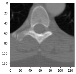
plt.imshow(65535 - ds.pixel_array, cmap='gray')
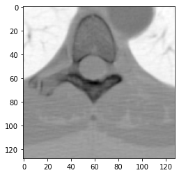
Tkinter と共に pydicom を使用する
contrib-pydicom レポジトリのプログラム pydicom_Tkinter.py は、殆どの Python インストールでデフォルトで装備される Tkinter グラフィクス・システムを使用して画像を表示する方法を実演します。それは Label ウィジェットかユーザ提供のウィジェットで Tkinter PhotoImage を作成します。
Python Imaging ライブラリ (PIL) と共に pydicom を使用する
contrib-pydicom レポジトリのモジュール pydicom_PIL.py は、pixel データとそれについての幾つかの基本的な情報 (bit depth, LUTs, etc) から Image インスタンスを作成した後、PIL の Image.show() メソッドを使用します。
wxPython と共に pydicom を使用する
contrib-pydicom レポジトリのモジュール imViewer-Simple.py は wxPython (PIL も、しかし厳密には必要ないかもしれないと記されています) を使用して pydicom データセットから画像を表示します。
以上
pydicom 2.2 : ユーザガイド : コア要素
pydicom 2.2 : ユーザガイド : コア要素 (翻訳/解説)
翻訳 : (株)クラスキャット セールスインフォメーション
作成日時 : 09/20/2021 (v2.2.1)
* 本ページは、pydicom の以下のドキュメントを翻訳した上で適宜、補足説明したものです:
- User Guide : Core elements in pydicom
* サンプルコードの動作確認はしておりますが、必要な場合には適宜、追加改変しています。
* ご自由にリンクを張って頂いてかまいませんが、sales-info@classcat.com までご一報いただけると嬉しいです。
- 人工知能研究開発支援
- 人工知能研修サービス(経営者層向けオンサイト研修)
- テクニカルコンサルティングサービス
- 実証実験(プロトタイプ構築)
- アプリケーションへの実装
- 人工知能研修サービス
- PoC(概念実証)を失敗させないための支援
- テレワーク & オンライン授業を支援
- お住まいの地域に関係なく Web ブラウザからご参加頂けます。事前登録 が必要ですのでご注意ください。
- ウェビナー運用には弊社製品「ClassCat® Webinar」を利用しています。
◆ お問合せ : 本件に関するお問い合わせ先は下記までお願いいたします。
| 株式会社クラスキャット セールス・マーケティング本部 セールス・インフォメーション |
| E-Mail:sales-info@classcat.com ; WebSite: https://www.classcat.com/ ; Facebook |
pydicom 2.2 : ユーザガイド : コア要素
Dataset は直接扱う主要オブジェクトです。Dataset は辞書をラップします、そこではキーは DICOM タグ (下で説明される、BaseTag オブジェクトとして) で、値は対応する DataElement インスタンス (これも下で説明されます) です。それは dict の殆どのメソッドを実装していますので、殆どの場合それはラップされた dict のように動作します。これは以下で示されるように、タグを介してデータ要素への直接アクセスを可能にします。
Dataset は直接作成できますが、通常は既存の DICOM ファイルを読むことにより取得します :
import pydicom
from pydicom.data import get_testdata_file
# get some test data
filename = get_testdata_file("rtplan.dcm")
ds = pydicom.dcmread(filename)
その文字列 (str() or reprt()) 値を単純にプリントすることによりデータセット全体を表示できます :
ds
Dataset.file_meta -------------------------------
(0002, 0000) File Meta Information Group Length  UL: 156
(0002, 0001) File Meta Information Version       OB: b'\x00\x01'
(0002, 0002) Media Storage SOP Class UID         UI: RT Plan Storage
(0002, 0003) Media Storage SOP Instance UID      UI: 1.2.999.999.99.9.9999.9999.20030903150023
(0002, 0010) Transfer Syntax UID                 UI: Implicit VR Little Endian
(0002, 0012) Implementation Class UID            UI: 1.2.888.888.88.8.8.8
-------------------------------------------------
(0008, 0012) Instance Creation Date              DA: '20030903'
(0008, 0013) Instance Creation Time              TM: '150031'
(0008, 0016) SOP Class UID                       UI: RT Plan Storage
(0008, 0018) SOP Instance UID                    UI: 1.2.777.777.77.7.7777.7777.20030903150023
(0008, 0020) Study Date                          DA: '20030716'
(0008, 0030) Study Time                          TM: '153557'
(0008, 0050) Accession Number                    SH: ''
(0008, 0060) Modality                            CS: 'RTPLAN'
(0008, 0070) Manufacturer                        LO: 'Manufacturer name here'
(0008, 0080) Institution Name                    LO: 'Here'
(0008, 0090) Referring Physician's Name          PN: ''
(0008, 1010) Station Name                        SH: 'COMPUTER002'
(0008, 1040) Institutional Department Name       LO: 'Radiation Therap'
(0008, 1070) Operators' Name                     PN: 'operator'
(0008, 1090) Manufacturer's Model Name           LO: 'Treatment Planning System name here'
(0010, 0010) Patient's Name                      PN: 'Last^First^mid^pre'
(0010, 0020) Patient ID                          LO: 'id00001'
(0010, 0030) Patient's Birth Date                DA: ''
(0010, 0040) Patient's Sex                       CS: 'O'
(0018, 1020) Software Versions                   LO: 'softwareV1'
(0020, 000d) Study Instance UID                  UI: 1.22.333.4.555555.6.7777777777777777777777777777
(0020, 000e) Series Instance UID                 UI: 1.2.333.444.55.6.7777.8888
(0020, 0010) Study ID                            SH: 'study1'
(0020, 0011) Series Number                       IS: '2'
(300a, 0002) RT Plan Label                       SH: 'Plan1'
(300a, 0003) RT Plan Name                        LO: 'Plan1'
(300a, 0006) RT Plan Date                        DA: '20030903'
(300a, 0007) RT Plan Time                        TM: '150023'
(300a, 000c) RT Plan Geometry                    CS: 'PATIENT'
(300a, 0010)  Dose Reference Sequence  2 item(s) ----
   (300a, 0012) Dose Reference Number               IS: '1'
   (300a, 0014) Dose Reference Structure Type       CS: 'COORDINATES'
   (300a, 0016) Dose Reference Description          LO: 'iso'
   (300a, 0018) Dose Reference Point Coordinates    DS: [239.531250000000, 239.531250000000, -741.87000000000]
   (300a, 0020) Dose Reference Type                 CS: 'ORGAN_AT_RISK'
   (300a, 0023) Delivery Maximum Dose               DS: '75.0'
   (300a, 002c) Organ at Risk Maximum Dose          DS: '75.0'
   ---------
   (300a, 0012) Dose Reference Number               IS: '2'
   (300a, 0014) Dose Reference Structure Type       CS: 'COORDINATES'
   (300a, 0016) Dose Reference Description          LO: 'PTV'
   (300a, 0018) Dose Reference Point Coordinates    DS: [239.531250000000, 239.531250000000, -751.87000000000]
   (300a, 0020) Dose Reference Type                 CS: 'TARGET'
   (300a, 0026) Target Prescription Dose            DS: '30.826203'
   ---------
(300a, 0070)  Fraction Group Sequence  1 item(s) ----
   (300a, 0071) Fraction Group Number               IS: '1'
   (300a, 0078) Number of Fractions Planned         IS: '30'
   (300a, 0080) Number of Beams                     IS: '1'
   (300a, 00a0) Number of Brachy Application Setups IS: '0'
   (300c, 0004)  Referenced Beam Sequence  1 item(s) ----
      (300a, 0082) Beam Dose Specification Point       DS: [239.531250000000, 239.531250000000, -751.87000000000]
      (300a, 0084) Beam Dose                           DS: '1.0275401'
      (300a, 0086) Beam Meterset                       DS: '116.0036697'
      (300c, 0006) Referenced Beam Number              IS: '1'
      ---------
   ---------
(300a, 00b0)  Beam Sequence  1 item(s) ----
   (0008, 0070) Manufacturer                        LO: 'Linac co.'
   (0008, 0080) Institution Name                    LO: 'Here'
   (0008, 1040) Institutional Department Name       LO: 'Radiation Therap'
   (0008, 1090) Manufacturer's Model Name           LO: 'Zapper9000'
   (0018, 1000) Device Serial Number                LO: '9999'
   (300a, 00b2) Treatment Machine Name              SH: 'unit001'
   (300a, 00b3) Primary Dosimeter Unit              CS: 'MU'
   (300a, 00b4) Source-Axis Distance                DS: '1000.0'
   (300a, 00b6)  Beam Limiting Device Sequence  2 item(s) ----
      (300a, 00b8) RT Beam Limiting Device Type        CS: 'X'
      (300a, 00bc) Number of Leaf/Jaw Pairs            IS: '1'
      ---------
      (300a, 00b8) RT Beam Limiting Device Type        CS: 'Y'
      (300a, 00bc) Number of Leaf/Jaw Pairs            IS: '1'
      ---------
   (300a, 00c0) Beam Number                         IS: '1'
   (300a, 00c2) Beam Name                           LO: 'Field 1'
   (300a, 00c4) Beam Type                           CS: 'STATIC'
   (300a, 00c6) Radiation Type                      CS: 'PHOTON'
   (300a, 00ce) Treatment Delivery Type             CS: 'TREATMENT'
   (300a, 00d0) Number of Wedges                    IS: '0'
   (300a, 00e0) Number of Compensators              IS: '0'
   (300a, 00ed) Number of Boli                      IS: '0'
   (300a, 00f0) Number of Blocks                    IS: '0'
   (300a, 010e) Final Cumulative Meterset Weight    DS: '1.0'
   (300a, 0110) Number of Control Points            IS: '2'
   (300a, 0111)  Control Point Sequence  2 item(s) ----
      (300a, 0112) Control Point Index                 IS: '0'
      (300a, 0114) Nominal Beam Energy                 DS: '6.0'
      (300a, 0115) Dose Rate Set                       DS: '650.0'
      (300a, 011a)  Beam Limiting Device Position Sequence  2 item(s) ----
         (300a, 00b8) RT Beam Limiting Device Type        CS: 'X'
         (300a, 011c) Leaf/Jaw Positions                  DS: [-100.00000000000, 100.000000000000]
         ---------
         (300a, 00b8) RT Beam Limiting Device Type        CS: 'Y'
         (300a, 011c) Leaf/Jaw Positions                  DS: [-100.00000000000, 100.000000000000]
         ---------
      (300a, 011e) Gantry Angle                        DS: '0.0'
      (300a, 011f) Gantry Rotation Direction           CS: 'NONE'
      (300a, 0120) Beam Limiting Device Angle          DS: '0.0'
      (300a, 0121) Beam Limiting Device Rotation Direc CS: 'NONE'
      (300a, 0122) Patient Support Angle               DS: '0.0'
      (300a, 0123) Patient Support Rotation Direction  CS: 'NONE'
      (300a, 0125) Table Top Eccentric Angle           DS: '0.0'
      (300a, 0126) Table Top Eccentric Rotation Direct CS: 'NONE'
      (300a, 0128) Table Top Vertical Position         DS: None
      (300a, 0129) Table Top Longitudinal Position     DS: None
      (300a, 012a) Table Top Lateral Position          DS: None
      (300a, 012c) Isocenter Position                  DS: [235.711172833292, 244.135437110782, -724.97815409918]
      (300a, 0130) Source to Surface Distance          DS: '898.429664831309'
      (300a, 0134) Cumulative Meterset Weight          DS: '0.0'
      (300c, 0050)  Referenced Dose Reference Sequence  2 item(s) ----
         (300a, 010c) Cumulative Dose Reference Coefficie DS: '0.0'
         (300c, 0051) Referenced Dose Reference Number    IS: '1'
         ---------
         (300a, 010c) Cumulative Dose Reference Coefficie DS: '0.0'
         (300c, 0051) Referenced Dose Reference Number    IS: '2'
         ---------
      ---------
      (300a, 0112) Control Point Index                 IS: '1'
      (300a, 0134) Cumulative Meterset Weight          DS: '1.0'
      (300c, 0050)  Referenced Dose Reference Sequence  2 item(s) ----
         (300a, 010c) Cumulative Dose Reference Coefficie DS: '0.9990268'
         (300c, 0051) Referenced Dose Reference Number    IS: '1'
         ---------
         (300a, 010c) Cumulative Dose Reference Coefficie DS: '1.0'
         (300c, 0051) Referenced Dose Reference Number    IS: '2'
         ---------
      ---------
   (300c, 006a) Referenced Patient Setup Number     IS: '1'
   ---------
(300a, 0180)  Patient Setup Sequence  1 item(s) ----
   (0018, 5100) Patient Position                    CS: 'HFS'
   (300a, 0182) Patient Setup Number                IS: '1'
   (300a, 01b2) Setup Technique Description         ST: ''
   ---------
(300c, 0002)  Referenced RT Plan Sequence  1 item(s) ----
   (0008, 1150) Referenced SOP Class UID            UI: RT Plan Storage
   (0008, 1155) Referenced SOP Instance UID         UI: 1.9.999.999.99.9.9999.9999.20030903145128
   (300a, 0055) RT Plan Relationship                CS: 'PREDECESSOR'
   ---------
(300c, 0060)  Referenced Structure Set Sequence  1 item(s) ----
   (0008, 1150) Referenced SOP Class UID            UI: RT Structure Set Storage
   (0008, 1155) Referenced SOP Instance UID         UI: 1.2.333.444.55.6.7777.88888
   ---------
(300e, 0002) Approval Status                     CS: 'UNAPPROVED'
Note : サンプルプログラム dcm_qt_tree.py を使用して DICOM ファイルを折り畳み式のツリーで見ることもできます。
DICOM キーワードやタグナンバーにより特定の要素にアクセスできます :
ds.PatientName
ds[0x10,0x10].value
'Last^First^mid^pre'
'Last^First^mid^pre'
タグナンバーを直接使用するとき DataElement インスタンスが返されますので、値を得るために DataElement.value が使用される必要があります。
Warning : pydicom では、private データ要素は名前を角括弧で囲んで表示されます (名前が pydicom に知れている場合)。これらは便宜上表示されているだけです ; 括弧内の記述的な名前はデータ要素を取得するためには使用できません。Private Data Elements の詳細を見てください。
要素のキーワードやタグナンバーを使用して要素の値を設定することもできます :
ds.PatientID = "12345"
ds.SeriesNumber = 5
ds[0x10,0x10].value = 'Test'
pydicom はメンバー変数のリクエストをインターセプトして、それらが DICOM 辞書にあるか確認しますので、名前の使用が可能です。それはキーワードを (group, element) タグに変換してそのタグの対応する値を (それがデータセットに存在すれば) 返します。
データ要素の削除と割当ての使用例については Anonymize DICOM data を参照してください。
Note : pydicom の Sequence の使用を理解するには、このオブジェクトモデルを参照してください :
- Dataset (Python dict をラップする)
- DataElement インスタンスを含みます、各要素の値は以下の一つです :
- int, float, str, bytes 等の通常の数値、文字列またはテキスト値
- 通常の値のリスト (e.g. a 三次元座標)
- Sequence インスタンス、ここで Sequence は Dataset インスタンスのリストです。
- Where each Dataset contains DataElement instances, and so on…
- DataElement インスタンスを含みます、各要素の値は以下の一つです :
シークエンス要素の値は Python リストをラップする Sequence インスタンスです。シークエンスの項目は Python の慣習のようにインデックス 0 で始まる、番号で参照されます。
ds.BeamSequence[0].BeamName
# Or, set an intermediate variable to a dataset in the list
beam1 = ds.BeamSequence[0]  # First dataset in the sequence
beam1.BeamName
'Field 1'
Working with sequences を参照してください。
DICOM キーワードの使用はデータ要素にアクセスするために推奨される方法ですが、以下のように、タグナンバーを直接使用することもできます :
# Same thing with tag numbers - much harder to read:
# Really should only be used if DICOM keyword not in pydicom dictionary
ds[0x300a,0xb0][0][0x300a,0xc2].value
'Field 1'
正確な要素タグやキーワードを覚えていないか知らない場合、Dataset は便利な Dataset.dir() メソッドを提供しています、対話的セッションの間 Python プロンプトで役立ちます :
ds.dir()
['AccessionNumber',
 'ApprovalStatus',
 'BeamSequence',
 'DoseReferenceSequence',
 'FractionGroupSequence',
 'InstanceCreationDate',
 'InstanceCreationTime',
 'InstitutionName',
 'InstitutionalDepartmentName',
 'Manufacturer',
 'ManufacturerModelName',
 'Modality',
 'OperatorsName',
 'PatientBirthDate',
 'PatientID',
 'PatientName',
 'PatientSetupSequence',
 'PatientSex',
 'RTPlanDate',
 'RTPlanGeometry',
 'RTPlanLabel',
 'RTPlanName',
 'RTPlanTime',
 'ReferencedRTPlanSequence',
 'ReferencedStructureSetSequence',
 'ReferringPhysicianName',
 'SOPClassUID',
 'SOPInstanceUID',
 'SeriesInstanceUID',
 'SeriesNumber',
 'SoftwareVersions',
 'StationName',
 'StudyDate',
 'StudyID',
 'StudyInstanceUID',
 'StudyTime']
ds.dir("pat")
['PatientBirthDate',
 'PatientID',
 'PatientName',
 'PatientSetupSequence',
 'PatientSex']
Dataset.dir() は、キーワード (case insensitive) で指定された文字列を任意の場所に持つ、データセット内部の非プライベート要素キーワードを返します。
Note : 引数を渡さずに Dataser.dir() を呼び出すとデータセットの総ての非プライベート要素キーワードのリストを返します。
_dicom_dict.py ファイルを参照することにより pydicom が知る総ての名前を見ることもできます。それは通常は必要ないはずですが、add_dict_entry() や add_dict_entries() を使用して独自のエントリを DICOM 辞書に実行時に追加することができます。同様に、using add_private_dict_entry() か add_private_dict_entries() を使用してプライベートデータ要素をプライベート辞書に追加できます。
内部的には、Dataset は各項目に対する DataElement オブジェクトをストアしますが、キーワード (e.g. ds.PatientName) によりアクセスされるときは DataElement の値だけが返されます。オブジェクト自身が必要な場合には、(公式 DICOM 要素のための) キーワードかタグナンバーのいずれかを使用して項目にアクセスできます。
# reload the data
ds = pydicom.dcmread(filename)
elem = ds['PatientName']
elem.VR, elem.value
# an alternative is to use:
elem = ds[0x0010,0x0010]
elem.VR, elem.value
('PN', 'Last^First^mid^pre')
Dataset が特定の要素を含むか確認するには要素のキーワードかタグで in 演算子を使用します :
"PatientName" in ds # or (0x0010,0x0010) in ds
True
Dataset から要素を削除するには del 演算子を使用します :
del ds.SoftwareVersions # or del ds[0x0018, 0x1020]
(7FE0,0010) Pixel Data を扱うには、PixelData キーワードで raw バイトが利用可能です :
# read data with actual pixel data
filename = get_testdata_file("CT_small.dcm")
ds = pydicom.dcmread(filename)
pixel_bytes = ds.PixelData
けれども numpy.ndarray を返す Dataset.pixel_array を使用するほうが遥かに便利です (NumPy ライブラリが必要です) :
arr = ds.pixel_array
arr
array([[175, 180, 166, ..., 203, 207, 216],
       [186, 183, 157, ..., 181, 190, 239],
       [184, 180, 171, ..., 152, 164, 235],
       ...,
       [906, 910, 923, ..., 922, 929, 927],
       [914, 954, 938, ..., 942, 925, 905],
       [959, 955, 916, ..., 911, 904, 909]], dtype=int16)
詳細は、Pixel データの操作 を参照してください。
DataElement
DataElement クラスは通常はユーザコードで直接使用されませんが、Dataset により広範に使用されます。DataElement は単純なオブジェクトで以下のものをストアします :
- タグ – 要素のタグ (BaseTag オブジェクトとして)
- VR – 要素の値表現 – 保存されている値の形式に表わす 2 文字 str
- VM – 要素の int としての多重性 (= Value Multiplicity)。これは value の内容から自動的に決定されます。
- value – 要素の実際の値。数字や文字列のような通常の値 (or VM > 1 ならばそれらのリスト)、または Sequence。
タグ
一般には Tag() はユーザコードでは直接使用されません、上記のセクションで示されたようにキーワードを使用して要素を割当てたり読むときに BaseTag が自動的に作成されるからです。
BaseTag クラスは int から派生してるので、実際には、幾つかの追加動作を伴う単なる数値です :
- Tag() は BaseTag のインスタンスを作成するために使用され、DICOM タグが想定される 4 バイト (group, element) に収まることを強制します。
- BaseTag インスタンスは int または (group,element) を含むタプルからか、DICOM キーワードから作成できます :
from pydicom.tag import Tag
t1 = Tag(0x00100010) # all of these are equivalent
t2 = Tag(0x10,0x10)
t3 = Tag((0x10, 0x10))
t4 = Tag("PatientName")
t1
type(t1)
t1==t2, t1==t3, t1==t4
(True, True, True)
- タグのグループと要素部分を返すための BaseTag.group と BaseTag.elem。
- BaseTag.is_private プロパティはタグがプライベート・タグを表わすか否か (i.e. グループ・ナンバーが奇数か) を確認します。
シークエンス
シークエンス は Python のリストから派生しています。追加された唯一の機能は文字列表現をより良くする (= prettier) ことです。それ以外の項目の選択、append 等のリストの通常の総てのメソッドは利用可能です。
以上
pydicom 2.2 : イントロダクション
pydicom 2.2 : イントロダクション(翻訳/解説)
翻訳 : (株)クラスキャット セールスインフォメーション
作成日時 : 09/20/2021 (v2.2.1)
* 本ページは、pydicom の以下のドキュメントを翻訳した上で適宜、補足説明したものです:
* サンプルコードの動作確認はしておりますが、必要な場合には適宜、追加改変しています。
* ご自由にリンクを張って頂いてかまいませんが、sales-info@classcat.com までご一報いただけると嬉しいです。
- 人工知能研究開発支援
- 人工知能研修サービス(経営者層向けオンサイト研修)
- テクニカルコンサルティングサービス
- 実証実験(プロトタイプ構築)
- アプリケーションへの実装
- 人工知能研修サービス
- PoC(概念実証)を失敗させないための支援
- テレワーク & オンライン授業を支援
- お住まいの地域に関係なく Web ブラウザからご参加頂けます。事前登録 が必要ですのでご注意ください。
- ウェビナー運用には弊社製品「ClassCat® Webinar」を利用しています。
◆ お問合せ : 本件に関するお問い合わせ先は下記までお願いいたします。
| 株式会社クラスキャット セールス・マーケティング本部 セールス・インフォメーション |
| E-Mail:sales-info@classcat.com ; WebSite: https://www.classcat.com/ ; Facebook |
pydicom 2.2 : イントロダクション
pydicom は医療画像、レポートと放射線治療オブジェクトのような DICOM ファイルを扱うための純粋な Python パッケージです。
pydicom はこれらの複雑なファイルを簡単な操作で自然な pythonic 構造に読むことを簡単にします。変更されたデータセットは再度 DICOM 形式ファイルに書くことができます。
ここに対話的セッションで pydicom を使用する簡単なサンプルがあります、放射線治療計画ファイルを読み、患者の設定を head-first-supine (仰臥位) から head-first-prone (腹臥位) に変更し、そして新しいファイルにセーブします。
import pydicom
from pydicom.data import get_testdata_file
filename = get_testdata_file("rtplan.dcm")
ds = pydicom.dcmread(filename)  # plan dataset
ds.PatientName
ds.dir("setup")  # get a list of tags with "setup" somewhere in the name
ds.PatientSetupSequence[0]
ds.PatientSetupSequence[0].PatientPosition = "HFP"
ds.save_as("rtplan2.dcm")
'Last^First^mid^pre'

['PatientSetupSequence']

(0018, 5100) Patient Position                    CS: 'HFS'
(300a, 0182) Patient Setup Number                IS: '1'
(300a, 01b2) Setup Technique Description         ST: ''
ds.PatientSetupSequence[0].PatientPosition = "HFP"
pydicom は DICOM サーバではなく (代わりに pynetdicom 参照)、主として画像を表示するためのものでもありません。Python コードで DICOM ファイルのデータ要素を操作させるために設計されています。
pydicom はインストールと使用が簡単で、 純粋な Python パッケージですから、Python が動作するところではどこでも動作するはずです。
一つの制限は圧縮された pixel データ (e.g. JPEG) は最初にそれを解凍する場合にのみ知的な方法で変更できることです。ひとたび解凍されれば、最初に解凍されたデータと同じ方法で変更できて DICOM ファイルに書き戻すことができます。
以上
pydicom 2.2 : README (概要)
pydicom 2.2 : README (概要) (翻訳/解説)
翻訳 : (株)クラスキャット セールスインフォメーション
作成日時 : 09/18/2021 (v2.2.1)
* 本ページは、pydicom の以下のドキュメントを翻訳した上で適宜、補足説明したものです:
* サンプルコードの動作確認はしておりますが、必要な場合には適宜、追加改変しています。
* ご自由にリンクを張って頂いてかまいませんが、sales-info@classcat.com までご一報いただけると嬉しいです。
![]()
pydicom 2.2 : 概要 (README)
pydicom は DICOM ファイルで作業するための純粋な Python パッケージです。それは簡単な “pythonic” 流儀で貴方が DICOM データを読み、変更して書くことを可能にします。
純粋な Python パッケージですから、pydicom は他の要件なしに Python が実行できる場所であればどこでも実行できますが、Pixel データで作業している場合には NumPy もインストールすることを勧めます。
DICOM networking のための Python ライブラリを探している場合には私達の別のプロジェクトに関心があるかもしません : pynetdicom。
インストール
pip の使用 :
pip install pydicom
conda の使用 :
conda install -c conda-forge pydicom
開発版のためのインストール手順を含む詳細は、インストールガイド を見てください。
ドキュメント
pydicom ユーザガイド、チュートリアル、サンプル と API リファレンス ドキュメントは GitHub ページ上の 現在のリリース と 開発版 の両方に対して利用可能です。
Pixel データ
圧縮されたそして非圧縮の Pixel データは常に バイト として読まれ、変更されて書かれることが可能です :
>>> from pydicom import dcmread
>>> from pydicom.data import get_testdata_file
>>> path = get_testdata_file("CT_small.dcm")
>>> ds = dcmread(path)
>>> type(ds.PixelData)

>>> len(ds.PixelData)
32768
>>> ds.PixelData[:2]
b'\xaf\x00'
NumPy がインストールされていれば、Pixel データは Dataset.pixel_array プロパティを使用して ndarray に変換できます :
>>> arr = ds.pixel_array
>>> arr.shape
(128, 128)
>>> arr
array([[175, 180, 166, ..., 203, 207, 216],
       [186, 183, 157, ..., 181, 190, 239],
       [184, 180, 171, ..., 152, 164, 235],
       ...,
       [906, 910, 923, ..., 922, 929, 927],
       [914, 954, 938, ..., 942, 925, 905],
       [959, 955, 916, ..., 911, 904, 909]], dtype=int16)
圧縮された Pixel データ
JPEG, JPEG-LS と JPEG 2000
JPEG 圧縮 Pixel データを ndarray に変換することは一つまたはそれ以上の追加の Python ライブラリのインストールを必要とします。どのライブラリが必要かの情報については、pixel データハンドラ・ドキュメント を参照してください。
RLE
RLE Pixel データをエンコードしてデコードするには NumPy を必要とするだけですが、それは非常に遅い可能性があります。プロセスを高速化するために 一つ以上の追加の Python ライブラリをインストールする ことを考えることを望むかもしれません。
サンプル
より多くの サンプル はドキュメントで利用可能です。
患者の ID を変更する
from pydicom import dcmread

ds = dcmread("/path/to/file.dcm")
# Edit the (0010,0020) 'Patient ID' element
ds.PatientID = "12345678"
ds.save_as("/path/to/file_updated.dcm")
Pixel データを表示する
NumPy と matplotlib を使用して :
import matplotlib.pyplot as plt
from pydicom import dcmread
from pydicom.data import get_testdata_file

# The path to a pydicom test dataset
path = get_testdata_file("CT_small.dcm")
ds = dcmread(path)
# `arr` is a numpy.ndarray
arr = ds.pixel_array

plt.imshow(arr, cmap="gray")
plt.show()
![]()
以上
ClassCat® Chatbot
人工知能開発支援
- テクニカルコンサルティングサービス
- 実証実験 (プロトタイプ構築)
- アプリケーションへの実装
- 人工知能研修サービス
クラスキャット
セールス・インフォメーション
E-Mail:sales-info@classcat.com