ホーム » sales-info の投稿 (ページ 4)
作者アーカイブ: sales-info
MONAI 0.7 : tutorials : モジュール – 3D 画像変換 (幾何学的変換)
MONAI 0.7 : tutorials : モジュール – 3D 画像変換 (幾何学的変換) (翻訳/解説)
翻訳 : (株)クラスキャット セールスインフォメーション
作成日時 : 10/15/2021 (0.7.0)
* 本ページは、MONAI の以下のドキュメントを翻訳した上で適宜、補足説明したものです:
* サンプルコードの動作確認はしておりますが、必要な場合には適宜、追加改変しています。
* ご自由にリンクを張って頂いてかまいませんが、sales-info@classcat.com までご一報いただけると嬉しいです。

- 人工知能研究開発支援
- 人工知能研修サービス(経営者層向けオンサイト研修)
- テクニカルコンサルティングサービス
- 実証実験(プロトタイプ構築)
- アプリケーションへの実装
- 人工知能研修サービス
- PoC(概念実証)を失敗させないための支援
- テレワーク & オンライン授業を支援
- お住まいの地域に関係なく Web ブラウザからご参加頂けます。事前登録 が必要ですのでご注意ください。
- ウェビナー運用には弊社製品「ClassCat® Webinar」を利用しています。
◆ お問合せ : 本件に関するお問い合わせ先は下記までお願いいたします。
| 株式会社クラスキャット セールス・マーケティング本部 セールス・インフォメーション |
| E-Mail:sales-info@classcat.com ; WebSite: https://www.classcat.com/ ; Facebook |
![]()
MONAI 0.7 : tutorials : モジュール – 3D 画像変換 (幾何学的変換)
このノートブックは volumetric 画像の変換を実演します。
このノートブックは 3D 画像のための MONAI の変換モジュールを紹介します。
環境のセットアップ
!python -c "import monai" || pip install -q "monai-weekly[nibabel]"
!python -c "import matplotlib" || pip install -q matplotlib
from monai.transforms import (
    AddChanneld,
    LoadImage,
    LoadImaged,
    Orientationd,
    Rand3DElasticd,
    RandAffined,
    Spacingd,
)
from monai.config import print_config
from monai.apps import download_and_extract
import numpy as np
import matplotlib.pyplot as plt
import tempfile
import shutil
import os
import glob
インポートのセットアップ
# Copyright 2020 MONAI Consortium
# Licensed under the Apache License, Version 2.0 (the "License");
# you may not use this file except in compliance with the License.
# You may obtain a copy of the License at
#     http://www.apache.org/licenses/LICENSE-2.0
# Unless required by applicable law or agreed to in writing, software
# distributed under the License is distributed on an "AS IS" BASIS,
# WITHOUT WARRANTIES OR CONDITIONS OF ANY KIND, either express or implied.
# See the License for the specific language governing permissions and
# limitations under the License.


print_config()
MONAI version: 0.4.0+721.g75b7a446
Numpy version: 1.21.2
Pytorch version: 1.10.0a0+3fd9dcf
MONAI flags: HAS_EXT = False, USE_COMPILED = False
MONAI rev id: 75b7a4462647bfbe9bc8e7d8e5bff1238b87990d

Optional dependencies:
Pytorch Ignite version: 0.4.6
Nibabel version: 3.2.1
scikit-image version: 0.18.3
Pillow version: 8.2.0
Tensorboard version: 2.6.0
gdown version: 3.13.1
TorchVision version: 0.11.0a0
tqdm version: 4.62.1
lmdb version: 1.2.1
psutil version: 5.8.0
pandas version: 1.3.3
einops version: 0.3.2
transformers version: 4.10.2

For details about installing the optional dependencies, please visit:
    https://docs.monai.io/en/latest/installation.html#installing-the-recommended-dependencies
データディレクトリのセットアップ
MONAI_DATA_DIRECTORY 環境変数でディレクトリを指定できます。これは結果をセーブしてダウンロードを再利用することを可能にします。指定されない場合、一時ディレクトリが使用されます。
directory = os.environ.get("MONAI_DATA_DIRECTORY")
root_dir = tempfile.mkdtemp() if directory is None else directory
print(f"root dir is: {root_dir}")
root dir is: /workspace/data/medical
データセットのダウンロード
データセットをダウンロードして展開します。データセットは http://medicaldecathlon.com/ に由来します。
resource = "https://msd-for-monai.s3-us-west-2.amazonaws.com/Task09_Spleen.tar"
md5 = "410d4a301da4e5b2f6f86ec3ddba524e"

compressed_file = os.path.join(root_dir, "Task09_Spleen.tar")
data_dir = os.path.join(root_dir, "Task09_Spleen")
if not os.path.exists(data_dir):
    download_and_extract(resource, compressed_file, root_dir, md5)
MSD 脾臓データセット・パスを設定する
以下は Task09_Spleen/imagesTr と Task09_Spleen/labelsTr からの画像とラベルをペアにグループ化します。
train_images = sorted(
    glob.glob(os.path.join(data_dir, "imagesTr", "*.nii.gz")))
train_labels = sorted(
    glob.glob(os.path.join(data_dir, "labelsTr", "*.nii.gz")))
data_dicts = [
    {"image": image_name, "label": label_name}
    for image_name, label_name in zip(train_images, train_labels)
]
train_data_dicts, val_data_dicts = data_dicts[:-9], data_dicts[-9:]
画像ファイル名は辞書のリストに体系化されます。
train_data_dicts[0]
{'image': '/workspace/data/medical/Task09_Spleen/imagesTr/spleen_10.nii.gz',
 'label': '/workspace/data/medical/Task09_Spleen/labelsTr/spleen_10.nii.gz'}
データ辞書のリスト, train_data_dicts は PyTorch のデータローダで使用できます。
例えば :
from torch.utils.data import DataLoader

data_loader = DataLoader(train_data_dicts)
for training_sample in data_loader:
    # run the deep learning training with training_sample
このチュートリアルの残りは、最終的に深層学習モデルにより消費される train_data_dict をデータ配列に変換する「変換」のセットを提示します。
NIfTI ファイルをロードする
MONAI の一つの設計上の選択は、それは高位ワークフロー・コンポーネントだけでなく、最小限機能する形で比較的低位の API も提供することです。
例えば、LoadImage クラスは基礎となる Nibabel 画像ローダの単純な呼び出し可能なラッパーです。幾つかの必要なシステムパラメータでローダを構築した後、NIfTI ファイル名と共にローダインスタンスを呼び出すと画像データ配列とアフィン情報やボクセル・サイズのようなメタデータを返します。
loader = LoadImage(dtype=np.float32)
image, metadata = loader(train_data_dicts[0]["image"])
print(f"input: {train_data_dicts[0]['image']}")
print(f"image shape: {image.shape}")
print(f"image affine:\n{metadata['affine']}")
print(f"image pixdim:\n{metadata['pixdim']}")
input: /workspace/data/medical/Task09_Spleen/imagesTr/spleen_10.nii.gz
image shape: (512, 512, 55)
image affine:
[[   0.97656202    0.            0.         -499.02319336]
 [   0.            0.97656202    0.         -499.02319336]
 [   0.            0.            5.            0.        ]
 [   0.            0.            0.            1.        ]]
image pixdim:
[1.       0.976562 0.976562 5.       0.       0.       0.       0.      ]
多くの場合、入力のグループを訓練サンプルとしてロードすることを望みます。例えば教師あり画像セグメンテーション・ネットワークの訓練は訓練サンプルとして画像とラベルのペアを必要とします。
入力のグループが一貫して前処理されることを保証するため、MONAI はまた最小限機能する変換のための辞書ベースのインターフェイスも提供します。
LoadImaged は LoadImage の対応する辞書ベース版です :
loader = LoadImaged(keys=("image", "label"))
data_dict = loader(train_data_dicts[0])
print(f"input:, {train_data_dicts[0]}")
print(f"image shape: {data_dict['image'].shape}")
print(f"label shape: {data_dict['label'].shape}")
print(f"image pixdim:\n{data_dict['image_meta_dict']['pixdim']}")
input:, {'image': '/workspace/data/medical/Task09_Spleen/imagesTr/spleen_10.nii.gz', 'label': '/workspace/data/medical/Task09_Spleen/labelsTr/spleen_10.nii.gz'}
image shape: (512, 512, 55)
label shape: (512, 512, 55)
image pixdim:
[1.       0.976562 0.976562 5.       0.       0.       0.       0.      ]
image, label = data_dict["image"], data_dict["label"]
plt.figure("visualize", (8, 4))
plt.subplot(1, 2, 1)
plt.title("image")
plt.imshow(image[:, :, 30], cmap="gray")
plt.subplot(1, 2, 2)
plt.title("label")
plt.imshow(label[:, :, 30])
plt.show()
![]()
チャネル次元を追加する
MONAI の画像変換の殆どは入力データが次の shape を持つことを仮定しています :
[num_channels, spatial_dim_1, spatial_dim_2, … ,spatial_dim_n]
(チャネル 1st は PyTorch で一般に使用されるので) それらが一貫して解釈できるためです 。
ここでは入力画像は shape (512, 512, 55) を持ちますが、これは受け入れられる shape ではありませんので (チャネル次元が欠落しています)、shape を更新するために呼び出される変換を作成します :
add_channel = AddChanneld(keys=["image", "label"])
datac_dict = add_channel(data_dict)
print(f"image shape: {datac_dict['image'].shape}")
image shape: (1, 512, 512, 55)
今は幾つかの強度と空間変換を行なう準備ができました。
一貫したボクセルサイズへの再サンプリング
入力ボリュームは異なるボクセルサイズを持つかもしれません。以下の変換はボリュームが (1.5, 1.5, 5.) mm ボクセルサイズを持つように正規化するために作成します。変換は data_dict[‘image.affine’] からの元のボクセルサイズを読むように設定されています、これは対応する NIfTI ファイルからのもので、LoadImaged により先にロードされます。
spacing = Spacingd(keys=["image", "label"], pixdim=(
    1.5, 1.5, 5.0), mode=("bilinear", "nearest"))
data_dict = spacing(datac_dict)
print(f"image shape: {data_dict['image'].shape}")
print(f"label shape: {data_dict['label'].shape}")
print(f"image affine after Spacing:\n{data_dict['image_meta_dict']['affine']}")
print(f"label affine after Spacing:\n{data_dict['label_meta_dict']['affine']}")
image shape: (1, 334, 334, 55)
label shape: (1, 334, 334, 55)
image affine after Spacing:
[[   1.5           0.            0.         -499.02319336]
 [   0.            1.5           0.         -499.02319336]
 [   0.            0.            5.            0.        ]
 [   0.            0.            0.            1.        ]]
label affine after Spacing:
[[   1.5           0.            0.         -499.02319336]
 [   0.            1.5           0.         -499.02319336]
 [   0.            0.            5.            0.        ]
 [   0.            0.            0.            1.        ]]
spacing の変更を追跡するため、data_dict は Spacingd により更新されました :
- image.original_affine キーが data_dict に追加されて、元のアフィンを記録します。
- image.affine キーは現在のアフィンを持つように更新されます。
image, label = data_dict["image"], data_dict["label"]
plt.figure("visualise", (8, 4))
plt.subplot(1, 2, 1)
plt.title("image")
plt.imshow(image[0, :, :, 30], cmap="gray")
plt.subplot(1, 2, 2)
plt.title("label")
plt.imshow(label[0, :, :, 30])
plt.show()
![]()
指定された軸コードへの再方向付け (= Reorientation)
時に総ての入力ボリュームを一貫した軸方向にすることが望ましいです。デフォルトの軸ラベルは Left (L), Right (R), Posterior (P), Anterior (A), Inferior (I), Superior (S) です。以下の変換はボリュームを ‘Posterior, Left, Inferior’ (PLI) 方向を持つように再方向付けるために作成されます :
orientation = Orientationd(keys=["image", "label"], axcodes="PLI")
data_dict = orientation(data_dict)
print(f"image shape: {data_dict['image'].shape}")
print(f"label shape: {data_dict['label'].shape}")
print(f"image affine after Spacing:\n{data_dict['image_meta_dict']['affine']}")
print(f"label affine after Spacing:\n{data_dict['label_meta_dict']['affine']}")
image shape: (1, 334, 334, 55)
label shape: (1, 334, 334, 55)
image affine after Spacing:
[[  0.          -1.5          0.           0.47680664]
 [ -1.5          0.           0.           0.47680664]
 [  0.           0.          -5.         270.        ]
 [  0.           0.           0.           1.        ]]
label affine after Spacing:
[[  0.          -1.5          0.           0.47680664]
 [ -1.5          0.           0.           0.47680664]
 [  0.           0.          -5.         270.        ]
 [  0.           0.           0.           1.        ]]
image, label = data_dict["image"], data_dict["label"]
plt.figure("visualise", (8, 4))
plt.subplot(1, 2, 1)
plt.title("image")
plt.imshow(image[0, :, :, 30], cmap="gray")
plt.subplot(1, 2, 2)
plt.title("label")
plt.imshow(label[0, :, :, 30])
plt.show()
![]()
ランダムなアフィン変換
以下のアフィン変換は (300, 300, 50) 画像パッチを出力するように定義されています。パッチの一は x, y と z 軸のそれぞれについて (-40, 40), (-40, 40), (-2, 2) の範囲でランダムに選択されます。変換は画像の中心に対して相対的です。3D 回転角度は z 軸周りに (-45, 45) 度、そして x と y 軸周りに 5 度からランダムに選択されます。ランダムなスケーリング因子は各軸に沿って (1.0 – 0.15, 1.0 + 0.15) からランダムに選択されます。
rand_affine = RandAffined(
    keys=["image", "label"],
    mode=("bilinear", "nearest"),
    prob=1.0,
    spatial_size=(300, 300, 50),
    translate_range=(40, 40, 2),
    rotate_range=(np.pi / 36, np.pi / 36, np.pi / 4),
    scale_range=(0.15, 0.15, 0.15),
    padding_mode="border",
)
rand_affine.set_random_state(seed=123)
元の画像の様々なランダム化されたバージョンを生成するためにこのセルを再実行できます。
affined_data_dict = rand_affine(data_dict)
print(f"image shape: {affined_data_dict['image'].shape}")

image, label = affined_data_dict["image"][0], affined_data_dict["label"][0]
plt.figure("visualise", (8, 4))
plt.subplot(1, 2, 1)
plt.title("image")
plt.imshow(image[:, :, 15], cmap="gray")
plt.subplot(1, 2, 2)
plt.title("label")
plt.imshow(label[:, :, 15])
plt.show()
image shape: (1, 300, 300, 50)
ランダムな elastic 変形
同様に、以下の elastic 変形は (300, 300, 10) 画像パッチを出力するように定義されています。画像はアフィン変換と elastic 変形の組み合わせから再サンプリングされます。sigma_range は変形の滑らかさを制御します (15 より大きいと CPU 上では遅くなる可能性があります)。magnitude_range は変形の振幅を制御します (500 より大きいと、画像が非現実的になります)。
rand_elastic = Rand3DElasticd(
    keys=["image", "label"],
    mode=("bilinear", "nearest"),
    prob=1.0,
    sigma_range=(5, 8),
    magnitude_range=(100, 200),
    spatial_size=(300, 300, 10),
    translate_range=(50, 50, 2),
    rotate_range=(np.pi / 36, np.pi / 36, np.pi),
    scale_range=(0.15, 0.15, 0.15),
    padding_mode="border",
)
rand_elastic.set_random_state(seed=123)
元の画像の様々なランダム化されたバージョンを生成するためにこのセルを再実行できます。
deformed_data_dict = rand_elastic(data_dict)
print(f"image shape: {deformed_data_dict['image'].shape}")

image, label = deformed_data_dict["image"][0], deformed_data_dict["label"][0]
plt.figure("visualise", (8, 4))
plt.subplot(1, 2, 1)
plt.title("image")
plt.imshow(image[:, :, 5], cmap="gray")
plt.subplot(1, 2, 2)
plt.title("label")
plt.imshow(label[:, :, 5])
plt.show()
image shape: (1, 300, 300, 10)
![]()
データディレクトリのクリーンアップ
一時ディレクトリが使用された場合にはディレクトリを削除します。
if directory is None:
    shutil.rmtree(root_dir)
以上
MONAI 0.7 : tutorials : 高速化 – MONAI 機能による高速訓練
MONAI 0.7 : tutorials : 高速化 – MONAI 機能による高速訓練 (翻訳/解説)
翻訳 : (株)クラスキャット セールスインフォメーション
作成日時 : 10/15/2021 (0.7.0)
* 本ページは、MONAI の以下のドキュメントを翻訳した上で適宜、補足説明したものです:
* サンプルコードの動作確認はしておりますが、必要な場合には適宜、追加改変しています。
* ご自由にリンクを張って頂いてかまいませんが、sales-info@classcat.com までご一報いただけると嬉しいです。
- 人工知能研究開発支援
- 人工知能研修サービス(経営者層向けオンサイト研修)
- テクニカルコンサルティングサービス
- 実証実験(プロトタイプ構築)
- アプリケーションへの実装
- 人工知能研修サービス
- PoC(概念実証)を失敗させないための支援
- テレワーク & オンライン授業を支援
- お住まいの地域に関係なく Web ブラウザからご参加頂けます。事前登録 が必要ですのでご注意ください。
- ウェビナー運用には弊社製品「ClassCat® Webinar」を利用しています。
◆ お問合せ : 本件に関するお問い合わせ先は下記までお願いいたします。
| 株式会社クラスキャット セールス・マーケティング本部 セールス・インフォメーション |
| E-Mail:sales-info@classcat.com ; WebSite: https://www.classcat.com/ ; Facebook |
MONAI 0.7 : tutorials : 高速化 – MONAI 機能による高速訓練
このドキュメントは、訓練パイプラインをプロファイルする方法、データセットを分析して適切なアルゴリズムを選択する方法、そしてシングル GPU、マルチ GPU 更にはマルチノードで GPU 利用を最適化する方法の詳細を紹介します。
このチュートリアルは PyTorch 訓練プログラムと MONAI 最適化訓練プログラムを示し、そしてパフォーマンスを比較します :
- AMP (Auto 混合精度)
- 決定論的変換のための CacheDataset
- データを GPU とキャッシュに移してから、GPU 上でランダムな変換を実行する。
- 軽量タスクではマルチスレッド化された ThreadDataLoader は PyTorch DataLoader よりも高速です。
- 通常の Dice 損失の代わりに MONAI DiceCE 損失を使用する。
- 通常の Adam optimizer の代わりに MONAI Novograd optimizer を使用する。
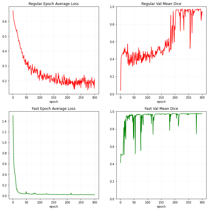
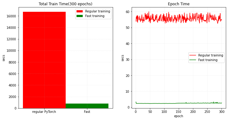
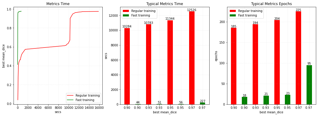
V100 GPU で、1 分内に 0.95 の検証平均 dice (損失) への訓練収束を獲得できます、それは同じメトリック達成するときの PyTorch の通常の実装と比べておよそ 200x 高速化しています。そして総てのエポックは通常の訓練よりも 20x 高速です。
それは 脾臓 3D セグメンテーション・チュートリアル ノートブックからの変更で、脾臓データセットは http://medicaldecathlon.com/ からダウンロードできます。
環境のセットアップ
!python -c "import monai" || pip install -q "monai-weekly[nibabel, tqdm]"
!python -c "import matplotlib" || pip install -q matplotlib
%matplotlib inline
インポートのセットアップ
# Copyright 2020 MONAI Consortium
# Licensed under the Apache License, Version 2.0 (the "License");
# you may not use this file except in compliance with the License.
# You may obtain a copy of the License at
#     http://www.apache.org/licenses/LICENSE-2.0
# Unless required by applicable law or agreed to in writing, software
# distributed under the License is distributed on an "AS IS" BASIS,
# WITHOUT WARRANTIES OR CONDITIONS OF ANY KIND, either express or implied.
# See the License for the specific language governing permissions and
# limitations under the License.

import glob
import math
import os
import shutil
import tempfile
import time

import matplotlib.pyplot as plt
import torch
from torch.optim import Adam
from monai.apps import download_and_extract
from monai.config import print_config
from monai.data import (
    CacheDataset,
    DataLoader,
    ThreadDataLoader,
    Dataset,
    decollate_batch,
)
from monai.inferers import sliding_window_inference
from monai.losses import DiceLoss, DiceCELoss
from monai.metrics import DiceMetric
from monai.networks.layers import Norm
from monai.networks.nets import UNet
from monai.optimizers import Novograd
from monai.transforms import (
    AddChanneld,
    AsDiscrete,
    Compose,
    CropForegroundd,
    FgBgToIndicesd,
    LoadImaged,
    Orientationd,
    RandCropByPosNegLabeld,
    ScaleIntensityRanged,
    Spacingd,
    ToDeviced,
    EnsureTyped,
    EnsureType,
)
from monai.utils import get_torch_version_tuple, set_determinism

print_config()

if get_torch_version_tuple() < (1, 6):
    raise RuntimeError(
        "AMP feature only exists in PyTorch version greater than v1.6."
    )
MONAI version: 0.2.0+1008.gf65d296f
Numpy version: 1.21.2
Pytorch version: 1.10.0a0+3fd9dcf
MONAI flags: HAS_EXT = False, USE_COMPILED = False
MONAI rev id: f65d296fe780f869dca84b6714dc36b94794930e

Optional dependencies:
Pytorch Ignite version: 0.4.5
Nibabel version: 3.2.1
scikit-image version: 0.18.3
Pillow version: 8.2.0
Tensorboard version: 2.6.0
gdown version: 3.13.0
TorchVision version: 0.11.0a0
tqdm version: 4.62.1
lmdb version: 1.2.1
psutil version: 5.8.0
pandas version: 1.3.2
einops version: 0.3.2
transformers version: NOT INSTALLED or UNKNOWN VERSION.

For details about installing the optional dependencies, please visit:
    https://docs.monai.io/en/latest/installation.html#installing-the-recommended-dependencies
データディレクトリのセットアップ
MONAI_DATA_DIRECTORY 環境変数でディレクトリを指定できます。これは結果をセーブしてダウンロードを再利用することを可能にします。指定されない場合、一時ディレクトリが使用されます。
directory = os.environ.get("MONAI_DATA_DIRECTORY")
root_dir = tempfile.mkdtemp() if directory is None else directory
print(f"root dir is: {root_dir}")
root dir is: /workspace/data/medical
データセットのダウンロード
Decathlon 脾臓データセットをダウンロードして展開します。
resource = "https://msd-for-monai.s3-us-west-2.amazonaws.com/Task09_Spleen.tar"
md5 = "410d4a301da4e5b2f6f86ec3ddba524e"

compressed_file = os.path.join(root_dir, "Task09_Spleen.tar")
data_root = os.path.join(root_dir, "Task09_Spleen")
if not os.path.exists(data_root):
    download_and_extract(resource, compressed_file, root_dir, md5)
MSD 脾臓データセット・パスの設定
train_images = sorted(
    glob.glob(os.path.join(data_root, "imagesTr", "*.nii.gz"))
)
train_labels = sorted(
    glob.glob(os.path.join(data_root, "labelsTr", "*.nii.gz"))
)
data_dicts = [
    {"image": image_name, "label": label_name}
    for image_name, label_name in zip(train_images, train_labels)
]
train_files, val_files = data_dicts[:-9], data_dicts[-9:]
訓練と検証のための変換のセットアップ
def transformations(fast=False):
    train_transforms = [
        LoadImaged(keys=["image", "label"]),
        AddChanneld(keys=["image", "label"]),
        Spacingd(
            keys=["image", "label"],
            pixdim=(1.5, 1.5, 2.0),
            mode=("bilinear", "nearest"),
        ),
        Orientationd(keys=["image", "label"], axcodes="RAS"),
        # change to execute transforms with Tensor data
        EnsureTyped(keys=["image", "label"]),
    ]
    if fast:
        # move the data to GPU and cache to avoid CPU -> GPU sync in every epoch
        train_transforms.append(
            ToDeviced(keys=["image", "label"], device="cuda:0")
        )
    train_transforms.extend([
        ScaleIntensityRanged(
            keys=["image"],
            a_min=-57,
            a_max=164,
            b_min=0.0,
            b_max=1.0,
            clip=True,
        ),
        CropForegroundd(keys=["image", "label"], source_key="image"),
        # pre-compute foreground and background indexes
        # and cache them to accelerate training
        FgBgToIndicesd(
            keys="label",
            fg_postfix="_fg",
            bg_postfix="_bg",
            image_key="image",
        ),
        # randomly crop out patch samples from big
        # image based on pos / neg ratio
        # the image centers of negative samples
        # must be in valid image area
        RandCropByPosNegLabeld(
            keys=["image", "label"],
            label_key="label",
            spatial_size=(96, 96, 96),
            pos=1,
            neg=1,
            num_samples=4,
            fg_indices_key="label_fg",
            bg_indices_key="label_bg",
        ),
    ])

    val_transforms = [
        LoadImaged(keys=["image", "label"]),
        AddChanneld(keys=["image", "label"]),
        Spacingd(
            keys=["image", "label"],
            pixdim=(1.5, 1.5, 2.0),
            mode=("bilinear", "nearest"),
        ),
        Orientationd(keys=["image", "label"], axcodes="RAS"),
        ScaleIntensityRanged(
            keys=["image"],
            a_min=-57,
            a_max=164,
            b_min=0.0,
            b_max=1.0,
            clip=True,
        ),
        CropForegroundd(keys=["image", "label"], source_key="image"),
        EnsureTyped(keys=["image", "label"]),
    ]
    if fast:
        # move the data to GPU and cache to avoid CPU -> GPU sync in every epoch
        val_transforms.append(
            ToDeviced(keys=["image", "label"], device="cuda:0")
        )

    return Compose(train_transforms), Compose(val_transforms)
訓練手順を定義する
典型的な PyTorch 通常の学習手続きについては、 モデルを訓練するために通常の Dataset, DataLoader, Adam optimizer と Dice 損失を使用します。
MONAI 高速訓練手順については、主として以下の機能を導入します :
- AMP (auto 混合精度): AMP は PyTorch v1.6 でリリースされた重要な機能で、NVIDIA CUDA 11 は AMP の強力なサポートを追加して訓練スピードを大幅に改善しました。
- CacheDataset: キャッシュ機構を持つ Dataset で、訓練の間にデータをロードして決定論的変換の結果をキャッシュできます。
- ToDeviced 変換: データを GPU に移して CacheDataset でキャッシュしてから、直接 GPU 上でランダムな変換を実行し、総てのエポックでの CPU -> GPU 同期を回避します。総ての MONAI 変換が GPU 演算をサポートはしてないことに注意してください、作業は進行中です。
- ThreadDataLoader: マルチプロセス処理の代わりにマルチスレッドを使用します、殆どの計算の結果を既にキャッシュしていますので軽量タスクでは DataLoader よりも高速です。
- Novograd optimizer: Novograd はペーパー "Stochastic Gradient Methods with Layer-wise Adaptive Moments for Training of Deep Networks" < https://arxiv.org/pdf/1905.11286.pdf > に基づいています。
- DiceCE 損失関数: Dice 損失と交差エントロピー損失を計算して、これら 2 つの損失の重み付けられた合計を返します。
def train_process(fast=False):
    max_epochs = 300
    learning_rate = 2e-4
    val_interval = 1  # do validation for every epoch

    train_trans, val_trans = transformations(fast=fast)
    # set CacheDataset, ThreadDataLoader and DiceCE loss for MONAI fast training
    if fast:
        train_ds = CacheDataset(
            data=train_files,
            transform=train_trans,
            cache_rate=1.0,
            num_workers=8,
        )
        val_ds = CacheDataset(
            data=val_files, transform=val_trans, cache_rate=1.0, num_workers=5
        )
        # disable multi-workers because `ThreadDataLoader` works with multi-threads
        train_loader = ThreadDataLoader(train_ds, num_workers=0, batch_size=4, shuffle=True)
        val_loader = ThreadDataLoader(val_ds, num_workers=0, batch_size=1)
        loss_function = DiceCELoss(to_onehot_y=True, softmax=True, squared_pred=True, batch=True)
    else:
        train_ds = Dataset(data=train_files, transform=train_trans)
        val_ds = Dataset(data=val_files, transform=val_trans)
        # num_worker=4 is the best parameter according to the test
        train_loader = DataLoader(train_ds, batch_size=4, shuffle=True, num_workers=4)
        val_loader = DataLoader(val_ds, batch_size=1, num_workers=4)
        loss_function = DiceLoss(to_onehot_y=True, softmax=True)

    device = torch.device("cuda:0")
    model = UNet(
        spatial_dims=3,
        in_channels=1,
        out_channels=2,
        channels=(16, 32, 64, 128, 256),
        strides=(2, 2, 2, 2),
        num_res_units=2,
        norm=Norm.BATCH,
    ).to(device)

    post_pred = Compose([EnsureType(), AsDiscrete(argmax=True, to_onehot=True, num_classes=2)])
    post_label = Compose([EnsureType(), AsDiscrete(to_onehot=True, num_classes=2)])

    dice_metric = DiceMetric(include_background=True, reduction="mean", get_not_nans=False)

    # set Novograd optimizer for MONAI training
    if fast:
        # Novograd paper suggests to use a bigger LR than Adam,
        # because Adam does normalization by element-wise second moments
        optimizer = Novograd(model.parameters(), learning_rate * 10)
        scaler = torch.cuda.amp.GradScaler()
    else:
        optimizer = Adam(model.parameters(), learning_rate)

    best_metric = -1
    best_metric_epoch = -1
    best_metrics_epochs_and_time = [[], [], []]
    epoch_loss_values = []
    metric_values = []
    epoch_times = []
    total_start = time.time()
    for epoch in range(max_epochs):
        epoch_start = time.time()
        print("-" * 10)
        print(f"epoch {epoch + 1}/{max_epochs}")
        model.train()
        epoch_loss = 0
        step = 0
        for batch_data in train_loader:
            step_start = time.time()
            step += 1
            inputs, labels = (
                batch_data["image"].to(device),
                batch_data["label"].to(device),
            )
            optimizer.zero_grad()
            # set AMP for MONAI training
            if fast:
                with torch.cuda.amp.autocast():
                    outputs = model(inputs)
                    loss = loss_function(outputs, labels)
                scaler.scale(loss).backward()
                scaler.step(optimizer)
                scaler.update()
            else:
                outputs = model(inputs)
                loss = loss_function(outputs, labels)
                loss.backward()
                optimizer.step()
            epoch_loss += loss.item()
            epoch_len = math.ceil(len(train_ds) / train_loader.batch_size)
            print(
                f"{step}/{epoch_len}, train_loss: {loss.item():.4f}"
                f" step time: {(time.time() - step_start):.4f}"
            )
        epoch_loss /= step
        epoch_loss_values.append(epoch_loss)
        print(f"epoch {epoch + 1} average loss: {epoch_loss:.4f}")

        if (epoch + 1) % val_interval == 0:
            model.eval()
            with torch.no_grad():
                for val_data in val_loader:
                    val_inputs, val_labels = (
                        val_data["image"].to(device),
                        val_data["label"].to(device),
                    )
                    roi_size = (160, 160, 160)
                    sw_batch_size = 4
                    # set AMP for MONAI validation
                    if fast:
                        with torch.cuda.amp.autocast():
                            val_outputs = sliding_window_inference(
                                val_inputs, roi_size, sw_batch_size, model
                            )
                    else:
                        val_outputs = sliding_window_inference(
                            val_inputs, roi_size, sw_batch_size, model
                        )
                    val_outputs = [post_pred(i) for i in decollate_batch(val_outputs)]
                    val_labels = [post_label(i) for i in decollate_batch(val_labels)]
                    dice_metric(y_pred=val_outputs, y=val_labels)

                metric = dice_metric.aggregate().item()
                dice_metric.reset()
                metric_values.append(metric)
                if metric > best_metric:
                    best_metric = metric
                    best_metric_epoch = epoch + 1
                    best_metrics_epochs_and_time[0].append(best_metric)
                    best_metrics_epochs_and_time[1].append(best_metric_epoch)
                    best_metrics_epochs_and_time[2].append(
                        time.time() - total_start
                    )
                    torch.save(model.state_dict(), "best_metric_model.pth")
                    print("saved new best metric model")
                print(
                    f"current epoch: {epoch + 1} current"
                    f" mean dice: {metric:.4f}"
                    f" best mean dice: {best_metric:.4f}"
                    f" at epoch: {best_metric_epoch}"
                )
        print(
            f"time consuming of epoch {epoch + 1} is:"
            f" {(time.time() - epoch_start):.4f}"
        )
        epoch_times.append(time.time() - epoch_start)

    total_time = time.time() - total_start
    print(
        f"train completed, best_metric: {best_metric:.4f}"
        f" at epoch: {best_metric_epoch}"
        f" total time: {total_time:.4f}"
    )
    return (
        max_epochs,
        epoch_loss_values,
        metric_values,
        epoch_times,
        best_metrics_epochs_and_time,
        total_time,
    )
決定論を有効にして通常の PyTorch 訓練を実行する
set_determinism(seed=0)
regular_start = time.time()
(
    epoch_num,
    epoch_loss_values,
    metric_values,
    epoch_times,
    best,
    train_time,
) = train_process(fast=False)
total_time = time.time() - regular_start
print(
    f"total time of {epoch_num} epochs with regular PyTorch training: {total_time:.4f}"
)
決定論を有効にして MONAI 最適化訓練を実行する
set_determinism(seed=0)
monai_start = time.time()
(
    epoch_num,
    m_epoch_loss_values,
    m_metric_values,
    m_epoch_times,
    m_best,
    m_train_time,
) = train_process(fast=True)
m_total_time = time.time() - monai_start
print(
    f"total time of {epoch_num} epochs with MONAI fast training: {m_train_time:.4f},"
    f" time of preparing cache: {(m_total_time - m_train_time):.4f}"
)
訓練損失と検証メトリクスをプロットする
plt.figure("train", (12, 12))
plt.subplot(2, 2, 1)
plt.title("Regular Epoch Average Loss")
x = [i + 1 for i in range(len(epoch_loss_values))]
y = epoch_loss_values
plt.xlabel("epoch")
plt.grid(alpha=0.4, linestyle=":")
plt.plot(x, y, color="red")

plt.subplot(2, 2, 2)
plt.title("Regular Val Mean Dice")
x = [i + 1 for i in range(len(metric_values))]
y = metric_values
plt.xlabel("epoch")
plt.ylim(0, 1)
plt.grid(alpha=0.4, linestyle=":")
plt.plot(x, y, color="red")

plt.subplot(2, 2, 3)
plt.title("Fast Epoch Average Loss")
x = [i + 1 for i in range(len(m_epoch_loss_values))]
y = m_epoch_loss_values
plt.xlabel("epoch")
plt.grid(alpha=0.4, linestyle=":")
plt.plot(x, y, color="green")

plt.subplot(2, 2, 4)
plt.title("Fast Val Mean Dice")
x = [i + 1 for i in range(len(m_metric_values))]
y = m_metric_values
plt.xlabel("epoch")
plt.ylim(0, 1)
plt.grid(alpha=0.4, linestyle=":")
plt.plot(x, y, color="green")
plt.show()
合計時間と総てのエポック時間をプロットする
plt.figure("train", (12, 6))
plt.subplot(1, 2, 1)
plt.title("Total Train Time(300 epochs)")
plt.bar(
    "regular PyTorch", total_time, 1, label="Regular training", color="red"
)
plt.bar("Fast", m_total_time, 1, label="Fast training", color="green")
plt.ylabel("secs")
plt.grid(alpha=0.4, linestyle=":")
plt.legend(loc="best")

plt.subplot(1, 2, 2)
plt.title("Epoch Time")
x = [i + 1 for i in range(len(epoch_times))]
plt.xlabel("epoch")
plt.ylabel("secs")
plt.plot(x, epoch_times, label="Regular training", color="red")
plt.plot(x, m_epoch_times, label="Fast training", color="green")
plt.grid(alpha=0.4, linestyle=":")
plt.legend(loc="best")
plt.show()
メトリクスを取得するための合計時間をプロットする
def get_best_metric_time(threshold, best_values):
    for i, v in enumerate(best_values[0]):
        if v > threshold:
            return best_values[2][i]
    return -1


def get_best_metric_epochs(threshold, best_values):
    for i, v in enumerate(best_values[0]):
        if v > threshold:
            return best_values[1][i]
    return -1


def get_label(index):
    if index == 0:
        return "Regular training"
    elif index == 1:
        return "Fast training"
    else:
        return None


plt.figure("train", (18, 6))
plt.subplot(1, 3, 1)
plt.title("Metrics Time")
plt.xlabel("secs")
plt.ylabel("best mean_dice")
plt.plot(best[2], best[0], label="Regular training", color="red")
plt.plot(m_best[2], m_best[0], label="Fast training", color="green")
plt.grid(alpha=0.4, linestyle=":")
plt.legend(loc="best")

plt.subplot(1, 3, 2)
plt.title("Typical Metrics Time")
plt.xlabel("best mean_dice")
plt.ylabel("secs")
labels = ["0.90", "0.90 ", "0.93", "0.93 ", "0.95", "0.95 ", "0.97", "0.97 "]
x_values = [0.9, 0.9, 0.93, 0.93, 0.95, 0.95, 0.97, 0.97]
for i, (l, x) in enumerate(zip(labels, x_values)):
    value = int(get_best_metric_time(x, best if i % 2 == 0 else m_best))
    color = "red" if i % 2 == 0 else "green"
    plt.bar(l, value, 0.5, label=get_label(i), color=color)
    plt.text(l, value, "%s" % value, ha="center", va="bottom")
plt.grid(alpha=0.4, linestyle=":")
plt.legend(loc="best")

plt.subplot(1, 3, 3)
plt.title("Typical Metrics Epochs")
plt.xlabel("best mean_dice")
plt.ylabel("epochs")
for i, (l, x) in enumerate(zip(labels, x_values)):
    value = int(get_best_metric_epochs(x, best if i % 2 == 0 else m_best))
    color = "red" if i % 2 == 0 else "green"
    plt.bar(l, value, 0.5, label=get_label(i), color=color)
    plt.text(l, value, "%s" % value, ha="center", va="bottom")
plt.grid(alpha=0.4, linestyle=":")
plt.legend(loc="best")
plt.show()
データディレクトリのクリーンアップ
一時ディレクトリが使用された場合にはディレクトリを削除します。
if directory is None:
    shutil.rmtree(root_dir)
以上
MONAI 0.7 : tutorials : モジュール – GAN ワークフロー・エンジン (配列版)
MONAI 0.7 : tutorials : モジュール – GAN ワークフロー・エンジン (配列版) (翻訳/解説)
翻訳 : (株)クラスキャット セールスインフォメーション
作成日時 : 10/14/2021 (0.7.0)
* 本ページは、MONAI の以下のドキュメントを翻訳した上で適宜、補足説明したものです:
* サンプルコードの動作確認はしておりますが、必要な場合には適宜、追加改変しています。
* ご自由にリンクを張って頂いてかまいませんが、sales-info@classcat.com までご一報いただけると嬉しいです。
- 人工知能研究開発支援
- 人工知能研修サービス(経営者層向けオンサイト研修)
- テクニカルコンサルティングサービス
- 実証実験(プロトタイプ構築)
- アプリケーションへの実装
- 人工知能研修サービス
- PoC(概念実証)を失敗させないための支援
- テレワーク & オンライン授業を支援
- お住まいの地域に関係なく Web ブラウザからご参加頂けます。事前登録 が必要ですのでご注意ください。
- ウェビナー運用には弊社製品「ClassCat® Webinar」を利用しています。
◆ お問合せ : 本件に関するお問い合わせ先は下記までお願いいたします。
| 株式会社クラスキャット セールス・マーケティング本部 セールス・インフォメーション |
| E-Mail:sales-info@classcat.com ; WebSite: https://www.classcat.com/ ; Facebook |
MONAI 0.7 : tutorials : モジュール – GAN ワークフロー・エンジン (配列版)
このノートブックは GanTrainer、モジュール化された敵対的学習のための MONAI ワークフロー・エンジンを示します。MedNIST ハンド CT スキャン・データセットを使用して医療画像再構築ネットワークを訓練します。配列バージョン。
MONAI フレームワークは敵対的生成ネットワークを簡単に設計し、訓練して評価するために使用できます。このノートブックは、ハンド CT スキャンの画像を再構築するために単純な GAN モデルを設計して訓練する MONAI コンポーネントを使用する実例を示します。
ネットワーク・アーキテクチャと損失関数についての詳細は MONAI Mednist GAN チュートリアル を読んでください。
Step 1: セットアップ
環境のセットアップ
!python -c "import monai" || pip install -q "monai-weekly[ignite, tqdm]"
!python -c "import matplotlib" || pip install -q matplotlib

%matplotlib inline
from monai.utils import set_determinism
from monai.transforms import (
    AddChannel,
    Compose,
    RandFlip,
    RandRotate,
    RandZoom,
    ScaleIntensity,
    EnsureType,
    Transform,
)
from monai.networks.nets import Discriminator, Generator
from monai.networks import normal_init
from monai.handlers import CheckpointSaver, MetricLogger, StatsHandler
from monai.engines.utils import GanKeys, default_make_latent
from monai.engines import GanTrainer
from monai.data import CacheDataset, DataLoader
from monai.config import print_config
from monai.apps import download_and_extract
import numpy as np
import torch
import matplotlib.pyplot as plt
import shutil
import sys
import logging
import tempfile
import os
インポートのセットアップ
print_config()
MONAI version: 0.6.0rc1+23.gc6793fd0
Numpy version: 1.20.3
Pytorch version: 1.9.0a0+c3d40fd
MONAI flags: HAS_EXT = True, USE_COMPILED = False
MONAI rev id: c6793fd0f316a448778d0047664aaf8c1895fe1c

Optional dependencies:
Pytorch Ignite version: 0.4.5
Nibabel version: 3.2.1
scikit-image version: 0.15.0
Pillow version: 7.0.0
Tensorboard version: 2.5.0
gdown version: 3.13.0
TorchVision version: 0.10.0a0
ITK version: 5.1.2
tqdm version: 4.53.0
lmdb version: 1.2.1
psutil version: 5.8.0
pandas version: 1.1.4
einops version: 0.3.0

For details about installing the optional dependencies, please visit:
    https://docs.monai.io/en/latest/installation.html#installing-the-recommended-dependencies
データディレクトリのセットアップ
MONAI_DATA_DIRECTORY 環境変数でディレクトリを指定できます。これは結果をセーブしてダウンロードを再利用することを可能にします。指定されない場合、一時ディレクトリが使用されます。
directory = os.environ.get("MONAI_DATA_DIRECTORY")
root_dir = tempfile.mkdtemp() if directory is None else directory
print(root_dir)
/workspace/data/medical
データセットをダウンロードする
データセットをダウンロードして展開します。
MedMNIST データセットは TCIA, RSNA Bone Age チャレンジ と NIH Chest X-ray データセット からの様々なセットから集められました。
データセットは Dr. Bradley J. Erickson M.D., Ph.D. (Department of Radiology, Mayo Clinic) のお陰により Creative Commons CC BY-SA 4.0 ライセンス のもとで利用可能になっています。
MedNIST データセットを使用する場合、出典を明示してください、e.g. https://github.com/Project-MONAI/tutorials/blob/master/2d_classification/mednist_tutorial.ipynb。
resource = "https://drive.google.com/uc?id=1QsnnkvZyJPcbRoV_ArW8SnE1OTuoVbKE"
md5 = "0bc7306e7427e00ad1c5526a6677552d"

compressed_file = os.path.join(root_dir, "MedNIST.tar.gz")
data_dir = os.path.join(root_dir, "MedNIST")
if not os.path.exists(data_dir):
    download_and_extract(resource, compressed_file, root_dir, md5)

hands = [
    os.path.join(data_dir, "Hand", x)
    for x in os.listdir(os.path.join(data_dir, "Hand"))
]
print(hands[:5])
['/workspace/data/medical/MedNIST/Hand/000317.jpeg', '/workspace/data/medical/MedNIST/Hand/002344.jpeg', '/workspace/data/medical/MedNIST/Hand/000816.jpeg', '/workspace/data/medical/MedNIST/Hand/004046.jpeg', '/workspace/data/medical/MedNIST/Hand/003316.jpeg']
Step 2: MONAI コンポーネントを初期化する
logging.basicConfig(stream=sys.stdout, level=logging.INFO)
set_determinism(0)
device = torch.device("cuda:0")
画像変換チェインを作成する
セーブされたディスク画像を利用可能なテンソルに変換するために処理パイプラインを定義します。
class LoadTarJpeg(Transform):
    def __call__(self, data):
        return plt.imread(data)


train_transforms = Compose(
    [
        LoadTarJpeg(),
        AddChannel(),
        ScaleIntensity(),
        RandRotate(range_x=np.pi / 12, prob=0.5, keep_size=True),
        RandFlip(spatial_axis=0, prob=0.5),
        RandZoom(min_zoom=0.9, max_zoom=1.1, prob=0.5),
        EnsureType(),
    ]
)
データセットとデーたローダを作成する
データを保持して訓練の間にバッチを提示します。
real_dataset = CacheDataset(hands, train_transforms)
100%|██████████| 10000/10000 [00:09<00:00, 1092.83it/s]
batch_size = 300
real_dataloader = DataLoader(
    real_dataset, batch_size=batch_size, shuffle=True, num_workers=10)

# We don't need to do any preparing so just return "as is"


def prepare_batch(batchdata, device=None, non_blocking=False):
    return batchdata.to(device=device, non_blocking=non_blocking)
generator と discriminator を定義する
基本的なコンピュータビジョン GAN ネットワークをライブラリからロードします。
# define networks
disc_net = Discriminator(
    in_shape=(1, 64, 64),
    channels=(8, 16, 32, 64, 1),
    strides=(2, 2, 2, 2, 1),
    num_res_units=1,
    kernel_size=5,
).to(device)

latent_size = 64
gen_net = Generator(
    latent_shape=latent_size,
    start_shape=(latent_size, 8, 8),
    channels=[32, 16, 8, 1],
    strides=[2, 2, 2, 1],
)
gen_net.conv.add_module("activation", torch.nn.Sigmoid())
gen_net = gen_net.to(device)

# initialize both networks
disc_net.apply(normal_init)
gen_net.apply(normal_init)

# define optimizors
learning_rate = 2e-4
betas = (0.5, 0.999)
disc_opt = torch.optim.Adam(disc_net.parameters(), learning_rate, betas=betas)
gen_opt = torch.optim.Adam(gen_net.parameters(), learning_rate, betas=betas)

# define loss functions
disc_loss_criterion = torch.nn.BCELoss()
gen_loss_criterion = torch.nn.BCELoss()
real_label = 1
fake_label = 0


def discriminator_loss(gen_images, real_images):
    real = real_images.new_full((real_images.shape[0], 1), real_label)
    gen = gen_images.new_full((gen_images.shape[0], 1), fake_label)

    realloss = disc_loss_criterion(disc_net(real_images), real)
    genloss = disc_loss_criterion(disc_net(gen_images.detach()), gen)

    return (genloss + realloss) / 2


def generator_loss(gen_images):
    output = disc_net(gen_images)
    cats = output.new_full(output.shape, real_label)
    return gen_loss_criterion(output, cats)
訓練ハンドラを作成する
モデル訓練の間に操作を実行します。
metric_logger = MetricLogger(
    loss_transform=lambda x: {
        GanKeys.GLOSS: x[GanKeys.GLOSS], GanKeys.DLOSS: x[GanKeys.DLOSS]},
    metric_transform=lambda x: x,
)

handlers = [
    StatsHandler(
        name="batch_training_loss",
        output_transform=lambda x: {
            GanKeys.GLOSS: x[GanKeys.GLOSS],
            GanKeys.DLOSS: x[GanKeys.DLOSS],
        },
    ),
    CheckpointSaver(
        save_dir=os.path.join(root_dir, "hand-gan"),
        save_dict={"g_net": gen_net, "d_net": disc_net},
        save_interval=10,
        save_final=True,
        epoch_level=True,
    ),
    metric_logger,
]
GanTrainer を作成する
敵対的学習のための MONAI ワークフロー・エンジン。GanTrainer によってコンポーネントはここで集められます。
Goodfellow et al. 2014 https://arxiv.org/abs/1406.2661 に基づいた訓練ループを使用します。
- ランダムな潜在コードから m 個の fakes を生成します。
- これらの fakes と現在のバッチ reals で D を更新します、d_train_steps 回反復されます。
- 新しいランダムな潜在コードから m fakes を生成します。
- discriminator フィードバックを使用してこれらの fakes で generator を更新します。
disc_train_steps = 5
max_epochs = 50

trainer = GanTrainer(
    device,
    max_epochs,
    real_dataloader,
    gen_net,
    gen_opt,
    generator_loss,
    disc_net,
    disc_opt,
    discriminator_loss,
    d_prepare_batch=prepare_batch,
    d_train_steps=disc_train_steps,
    g_update_latents=True,
    latent_shape=latent_size,
    key_train_metric=None,
    train_handlers=handlers,
)
Step 3: 訓練の開始
trainer.run()
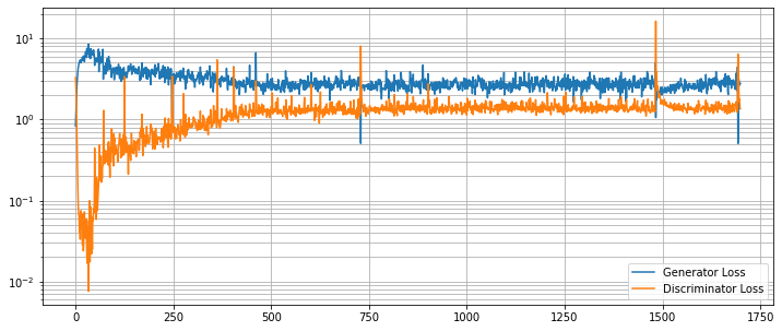
結果を評価する
G と D の損失カーブを崩れていないか調べます。
g_loss = [loss[1][GanKeys.GLOSS] for loss in metric_logger.loss]
d_loss = [loss[1][GanKeys.DLOSS] for loss in metric_logger.loss]
plt.figure(figsize=(12, 5))
plt.semilogy(g_loss, label="Generator Loss")
plt.semilogy(d_loss, label="Discriminator Loss")
plt.grid(True, "both", "both")
plt.legend()
plt.show()
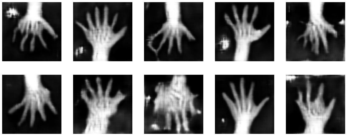
画像再構築を見る
ランダムな潜在コードで訓練された generator の出力を見ます。
test_img_count = 10
test_latents = default_make_latent(test_img_count, latent_size).to(device)
fakes = gen_net(test_latents)

fig, axs = plt.subplots(2, (test_img_count // 2), figsize=(20, 8))
axs = axs.flatten()
for i, ax in enumerate(axs):
    ax.axis("off")
    ax.imshow(fakes[i, 0].cpu().data.numpy(), cmap="gray")
データディレクトリのクリーンアップ
一時ディレクトリが作成された場合にはディレクトリを削除します。
if directory is None:
    shutil.rmtree(root_dir)
以上
MONAI 0.7 : tutorials : モジュール – GAN ワークフロー・エンジン (辞書版)
MONAI 0.7 : tutorials : モジュール – GAN ワークフロー・エンジン (辞書版) (翻訳/解説)
翻訳 : (株)クラスキャット セールスインフォメーション
作成日時 : 10/14/2021 (0.7.0)
* 本ページは、MONAI の以下のドキュメントを翻訳した上で適宜、補足説明したものです:
* サンプルコードの動作確認はしておりますが、必要な場合には適宜、追加改変しています。
* ご自由にリンクを張って頂いてかまいませんが、sales-info@classcat.com までご一報いただけると嬉しいです。
- 人工知能研究開発支援
- 人工知能研修サービス(経営者層向けオンサイト研修)
- テクニカルコンサルティングサービス
- 実証実験(プロトタイプ構築)
- アプリケーションへの実装
- 人工知能研修サービス
- PoC(概念実証)を失敗させないための支援
- テレワーク & オンライン授業を支援
- お住まいの地域に関係なく Web ブラウザからご参加頂けます。事前登録 が必要ですのでご注意ください。
- ウェビナー運用には弊社製品「ClassCat® Webinar」を利用しています。
◆ お問合せ : 本件に関するお問い合わせ先は下記までお願いいたします。
| 株式会社クラスキャット セールス・マーケティング本部 セールス・インフォメーション |
| E-Mail:sales-info@classcat.com ; WebSite: https://www.classcat.com/ ; Facebook |
MONAI 0.7 : tutorials : モジュール – GAN ワークフロー・エンジン (辞書版)
このノートブックは GanTrainer、モジュール化された敵対的学習のための MONAI ワークフロー・エンジンを示します。MedNIST ハンド CT スキャン・データセットを使用して医療画像再構築ネットワークを訓練します。辞書バージョン。
MONAI フレームワークは敵対的生成ネットワークを簡単に設計し、訓練して評価するために使用できます。このノートブックは、ハンド CT スキャンの画像を再構築するために単純な GAN モデルを設計して訓練する MONAI コンポーネントを使用する実例を示します。
ネットワーク・アーキテクチャと損失関数についての詳細は MONAI Mednist GAN チュートリアル を読んでください。
Step 1: セットアップ
環境のセットアップ
!python -c "import monai" || pip install -q "monai-weekly[ignite, tqdm]"
!python -c "import matplotlib" || pip install -q matplotlib
%matplotlib inline
from monai.utils import set_determinism
from monai.transforms import (
    AddChannelD,
    Compose,
    LoadImageD,
    RandFlipD,
    RandRotateD,
    RandZoomD,
    ScaleIntensityD,
    EnsureTypeD,
)
from monai.networks.nets import Discriminator, Generator
from monai.networks import normal_init
from monai.handlers import CheckpointSaver, MetricLogger, StatsHandler
from monai.engines.utils import GanKeys, default_make_latent
from monai.engines import GanTrainer
from monai.data import CacheDataset, DataLoader
from monai.config import print_config
from monai.apps import download_and_extract
import numpy as np
import torch
import matplotlib.pyplot as plt
import tempfile
import sys
import shutil
import os
import logging
インポートのセットアップ
print_config()
MONAI version: 0.6.0rc1+23.gc6793fd0
Numpy version: 1.20.3
Pytorch version: 1.9.0a0+c3d40fd
MONAI flags: HAS_EXT = True, USE_COMPILED = False
MONAI rev id: c6793fd0f316a448778d0047664aaf8c1895fe1c

Optional dependencies:
Pytorch Ignite version: 0.4.5
Nibabel version: 3.2.1
scikit-image version: 0.15.0
Pillow version: 7.0.0
Tensorboard version: 2.5.0
gdown version: 3.13.0
TorchVision version: 0.10.0a0
ITK version: 5.1.2
tqdm version: 4.53.0
lmdb version: 1.2.1
psutil version: 5.8.0
pandas version: 1.1.4
einops version: 0.3.0

For details about installing the optional dependencies, please visit:
    https://docs.monai.io/en/latest/installation.html#installing-the-recommended-dependencies
データディレクトリのセットアップ
MONAI_DATA_DIRECTORY 環境変数でディレクトリを指定できます。これは結果をセーブしてダウンロードを再利用することを可能にします。指定されない場合、一時ディレクトリが使用されます。
directory = os.environ.get("MONAI_DATA_DIRECTORY")
root_dir = tempfile.mkdtemp() if directory is None else directory
print(root_dir)
/workspace/data/medical
データセットをダウンロードする
データセットをダウンロードして展開します。
MedMNIST データセットは TCIA, RSNA Bone Age チャレンジ と NIH Chest X-ray データセット からの様々なセットから集められました。
データセットは Dr. Bradley J. Erickson M.D., Ph.D. (Department of Radiology, Mayo Clinic) のお陰により Creative Commons CC BY-SA 4.0 ライセンス のもとで利用可能になっています。
MedNIST データセットを使用する場合、出典を明示してください、e.g. https://github.com/Project-MONAI/tutorials/blob/master/2d_classification/mednist_tutorial.ipynb。
resource = "https://drive.google.com/uc?id=1QsnnkvZyJPcbRoV_ArW8SnE1OTuoVbKE"
md5 = "0bc7306e7427e00ad1c5526a6677552d"

compressed_file = os.path.join(root_dir, "MedNIST.tar.gz")
data_dir = os.path.join(root_dir, "MedNIST")
if not os.path.exists(data_dir):
    download_and_extract(resource, compressed_file, root_dir, md5)
hand_dir = os.path.join(data_dir, "Hand")
training_datadict = [
    {"hand": os.path.join(hand_dir, filename)}
    for filename in os.listdir(hand_dir)
]
print(training_datadict[:5])
[{'hand': '/workspace/data/medical/MedNIST/Hand/000317.jpeg'}, {'hand': '/workspace/data/medical/MedNIST/Hand/002344.jpeg'}, {'hand': '/workspace/data/medical/MedNIST/Hand/000816.jpeg'}, {'hand': '/workspace/data/medical/MedNIST/Hand/004046.jpeg'}, {'hand': '/workspace/data/medical/MedNIST/Hand/003316.jpeg'}]
Step 2: MONAI コンポーネントを初期化する
logging.basicConfig(stream=sys.stdout, level=logging.INFO)
set_determinism(0)
device = torch.device("cuda:0")
画像変換チェインを作成する
セーブされたディスク画像を利用可能なテンソルに変換するために処理パイプラインを定義します。
train_transforms = Compose(
    [
        LoadImageD(keys=["hand"]),
        AddChannelD(keys=["hand"]),
        ScaleIntensityD(keys=["hand"]),
        RandRotateD(keys=["hand"], range_x=np.pi /
                    12, prob=0.5, keep_size=True),
        RandFlipD(keys=["hand"], spatial_axis=0, prob=0.5),
        RandZoomD(keys=["hand"], min_zoom=0.9, max_zoom=1.1, prob=0.5),
        EnsureTypeD(keys=["hand"]),
    ]
)
データセットとデーたローダを作成する
データを保持して訓練の間にバッチを提示します。
real_dataset = CacheDataset(training_datadict, train_transforms)
100%|██████████| 10000/10000 [00:09<00:00, 1000.72it/s]
batch_size = 300
real_dataloader = DataLoader(
    real_dataset, batch_size=batch_size, shuffle=True, num_workers=10)


def prepare_batch(batchdata, device=None, non_blocking=False):
    return batchdata["hand"].to(device=device, non_blocking=non_blocking)
generator と discriminator を定義する
基本的なコンピュータビジョン GAN ネットワークをライブラリからロードします。
# define networks
disc_net = Discriminator(
    in_shape=(1, 64, 64),
    channels=(8, 16, 32, 64, 1),
    strides=(2, 2, 2, 2, 1),
    num_res_units=1,
    kernel_size=5,
).to(device)

latent_size = 64
gen_net = Generator(
    latent_shape=latent_size,
    start_shape=(latent_size, 8, 8),
    channels=[32, 16, 8, 1],
    strides=[2, 2, 2, 1],
)
gen_net.conv.add_module("activation", torch.nn.Sigmoid())
gen_net = gen_net.to(device)

# initialize both networks
disc_net.apply(normal_init)
gen_net.apply(normal_init)

# define optimizors
learning_rate = 2e-4
betas = (0.5, 0.999)
disc_opt = torch.optim.Adam(disc_net.parameters(), learning_rate, betas=betas)
gen_opt = torch.optim.Adam(gen_net.parameters(), learning_rate, betas=betas)

# define loss functions
disc_loss_criterion = torch.nn.BCELoss()
gen_loss_criterion = torch.nn.BCELoss()
real_label = 1
fake_label = 0


def discriminator_loss(gen_images, real_images):
    real = real_images.new_full((real_images.shape[0], 1), real_label)
    gen = gen_images.new_full((gen_images.shape[0], 1), fake_label)

    realloss = disc_loss_criterion(disc_net(real_images), real)
    genloss = disc_loss_criterion(disc_net(gen_images.detach()), gen)

    return (genloss + realloss) / 2


def generator_loss(gen_images):
    output = disc_net(gen_images)
    cats = output.new_full(output.shape, real_label)
    return gen_loss_criterion(output, cats)
訓練ハンドラを作成する
モデル訓練の間に操作を実行します。
metric_logger = MetricLogger(
    loss_transform=lambda x: {
        GanKeys.GLOSS: x[GanKeys.GLOSS], GanKeys.DLOSS: x[GanKeys.DLOSS]},
    metric_transform=lambda x: x,
)

handlers = [
    StatsHandler(
        name="batch_training_loss",
        output_transform=lambda x: {
            GanKeys.GLOSS: x[GanKeys.GLOSS],
            GanKeys.DLOSS: x[GanKeys.DLOSS],
        },
    ),
    CheckpointSaver(
        save_dir=os.path.join(root_dir, "hand-gan"),
        save_dict={"g_net": gen_net, "d_net": disc_net},
        save_interval=10,
        save_final=True,
        epoch_level=True,
    ),
    metric_logger,
]
GanTrainer を作成する
敵対的学習のための MONAI ワークフロー・エンジン。GanTrainer によってコンポーネントはここで集められます。
Goodfellow et al. 2014 https://arxiv.org/abs/1406.2661 に基づいた訓練ループを使用します。
- ランダムな潜在コードから m 個の fakes を生成します。
- これらの fakes と現在のバッチ reals で D を更新します、d_train_steps 回反復されます。
- 新しいランダムな潜在コードから m fakes を生成します。
- discriminator フィードバックを使用してこれらの fakes で generator を更新します。
disc_train_steps = 5
max_epochs = 50

trainer = GanTrainer(
    device,
    max_epochs,
    real_dataloader,
    gen_net,
    gen_opt,
    generator_loss,
    disc_net,
    disc_opt,
    discriminator_loss,
    d_prepare_batch=prepare_batch,
    d_train_steps=disc_train_steps,
    g_update_latents=True,
    latent_shape=latent_size,
    key_train_metric=None,
    train_handlers=handlers,
)
Step 3: 訓練の開始
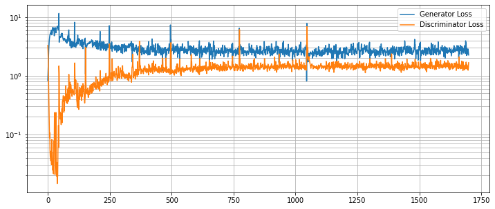
trainer.run()
結果を評価する
G と D の損失カーブを崩れていないか調べます。
g_loss = [loss[1][GanKeys.GLOSS] for loss in metric_logger.loss]
d_loss = [loss[1][GanKeys.DLOSS] for loss in metric_logger.loss]
plt.figure(figsize=(12, 5))
plt.semilogy(g_loss, label="Generator Loss")
plt.semilogy(d_loss, label="Discriminator Loss")
plt.grid(True, "both", "both")
plt.legend()
plt.show()
画像再構築を見る
ランダムな潜在コードで訓練された generator の出力を見ます。
test_img_count = 10
test_latents = default_make_latent(test_img_count, latent_size).to(device)
fakes = gen_net(test_latents)

fig, axs = plt.subplots(2, (test_img_count // 2), figsize=(20, 8))
axs = axs.flatten()
for i, ax in enumerate(axs):
    ax.axis("off")
    ax.imshow(fakes[i, 0].cpu().data.numpy(), cmap="gray")
データディレクトリのクリーンアップ
一時ディレクトリが作成された場合にはディレクトリを削除します。
if directory is None:
    shutil.rmtree(root_dir)
以上
MONAI 0.7 : tutorials : モジュール – 最適な学習率
MONAI 0.7 : tutorials : モジュール – 最適な学習率 (翻訳/解説)
翻訳 : (株)クラスキャット セールスインフォメーション
作成日時 : 10/13/2021 (0.7.0)
* 本ページは、MONAI の以下のドキュメントを翻訳した上で適宜、補足説明したものです:
* サンプルコードの動作確認はしておりますが、必要な場合には適宜、追加改変しています。
* ご自由にリンクを張って頂いてかまいませんが、sales-info@classcat.com までご一報いただけると嬉しいです。
- 人工知能研究開発支援
- 人工知能研修サービス(経営者層向けオンサイト研修)
- テクニカルコンサルティングサービス
- 実証実験(プロトタイプ構築)
- アプリケーションへの実装
- 人工知能研修サービス
- PoC(概念実証)を失敗させないための支援
- テレワーク & オンライン授業を支援
- お住まいの地域に関係なく Web ブラウザからご参加頂けます。事前登録 が必要ですのでご注意ください。
- ウェビナー運用には弊社製品「ClassCat® Webinar」を利用しています。
◆ お問合せ : 本件に関するお問い合わせ先は下記までお願いいたします。
| 株式会社クラスキャット セールス・マーケティング本部 セールス・インフォメーション |
| E-Mail:sales-info@classcat.com ; WebSite: https://www.classcat.com/ ; Facebook |
MONAI 0.7 : tutorials : モジュール – 最適な学習率
このノートブックは、ネットワークの学習率の値を調整するために LearningRateFinder を使用する方法を実演します。
このチュートリアルでは、MONAI の LearningRateFinder を調べるために MedNIST データセットを使用し、学習率の初期推定値を取得するためにそれを使用します。
そして最適化の過程で学習率を変化させるために PyTorch の周期的な学習率スケジューラの一つを採用します。これは改善された結果を与えることが示されています : https://arxiv.org/abs/1506.01186。これを optimizer (ADAM) のデフォルトの学習率と LearningRateFinder により提案された学習率と比較します。
この 2D 分類は非常に簡単ですので、それを少し難しく (そして高速に) するため、小さいネットワーク、画像のサブセットだけを使用し (訓練と検証のためにそれぞれ ~250 と ~25)、画像をクロップして (64×64 から 20×20 に) どのようなランダム変換も使用しません。より難しいシナリオでは、多分これらのどれも行なわないことを望むでしょう。
環境のセットアップ
!python -c "import monai" || pip install -q "monai-weekly[pillow, tqdm]"
!python -c "import matplotlib" || pip install -q matplotlib
インポートのセットアップ
# Copyright 2020 MONAI Consortium
# Licensed under the Apache License, Version 2.0 (the "License");
# you may not use this file except in compliance with the License.
# You may obtain a copy of the License at
#     http://www.apache.org/licenses/LICENSE-2.0
# Unless required by applicable law or agreed to in writing, software
# distributed under the License is distributed on an "AS IS" BASIS,
# WITHOUT WARRANTIES OR CONDITIONS OF ANY KIND, either express or implied.
# See the License for the specific language governing permissions and
# limitations under the License.

import os
import shutil
import tempfile

import matplotlib.pyplot as plt
import numpy as np
import torch
from monai.apps import MedNISTDataset
from monai.config import print_config
from monai.data import decollate_batch
from monai.metrics import ROCAUCMetric
from monai.networks.nets import DenseNet
from monai.networks.utils import eval_mode
from monai.optimizers import LearningRateFinder
from monai.transforms import (
    Activations,
    AsDiscrete,
    AddChanneld,
    CenterSpatialCropd,
    Compose,
    LoadImaged,
    ScaleIntensityd,
    EnsureTyped,
    EnsureType,
)
from monai.utils import set_determinism
from torch.utils.data import DataLoader
from tqdm import trange

print_config()
MONAI version: 0.6.0+1.g8365443a
Numpy version: 1.20.3
Pytorch version: 1.9.0a0+c3d40fd
MONAI flags: HAS_EXT = True, USE_COMPILED = False
MONAI rev id: 8365443ababac313340467e5987c7babe2b5b86a

Optional dependencies:
Pytorch Ignite version: 0.4.5
Nibabel version: 3.2.1
scikit-image version: 0.15.0
Pillow version: 8.2.0
Tensorboard version: 2.2.0
gdown version: 3.13.0
TorchVision version: 0.10.0a0
ITK version: 5.1.2
tqdm version: 4.53.0
lmdb version: 1.2.1
psutil version: 5.8.0
pandas version: 1.1.4
einops version: 0.3.0

For details about installing the optional dependencies, please visit:
    https://docs.monai.io/en/latest/installation.html#installing-the-recommended-dependencies
データディレクトリのセットアップ
MONAI_DATA_DIRECTORY 環境変数でディレクトリを指定できます。これは結果をセーブしてダウンロードを再利用することを可能にします。指定されない場合、一時ディレクトリが使用されます。
directory = os.environ.get("MONAI_DATA_DIRECTORY")
root_dir = tempfile.mkdtemp() if directory is None else directory
print(root_dir)
再現性のために決定論的訓練を設定する
set_determinism(seed=0)
MONAI 変換を定義してデータセットとデーたローダを取得する
transforms = Compose(
    [
        LoadImaged(keys="image"),
        AddChanneld(keys="image"),
        ScaleIntensityd(keys="image"),
        CenterSpatialCropd(keys="image", roi_size=(20, 20)),
        EnsureTyped(keys="image"),
    ]
)
# Set fraction of images used for testing to be very high, then don't use it. In this way, we can reduce the number
# of images in both train and val. Makes it faster and makes the training a little harder.
def get_data(section):
    ds = MedNISTDataset(
        root_dir=root_dir,
        transform=transforms,
        section=section,
        download=True,
        num_workers=10,
        val_frac=0.0005,
        test_frac=0.995,
    )
    loader = DataLoader(ds, batch_size=30, shuffle=True, num_workers=10)
    return ds, loader


train_ds, train_loader = get_data("training")
val_ds, val_loader = get_data("validation")

print(len(train_ds))
print(len(val_ds))
print(train_ds[0]["image"].shape)
num_classes = train_ds.get_num_classes()

y_pred_trans = Compose([EnsureType(), Activations(softmax=True)])
y_trans = Compose([EnsureType(), AsDiscrete(to_onehot=True, num_classes=num_classes)])
Verified 'MedNIST.tar.gz', md5: 0bc7306e7427e00ad1c5526a6677552d.
file /home/rbrown/data/MONAI/MedNIST.tar.gz exists, skip downloading.
extracted file /home/rbrown/data/MONAI/MedNIST exists, skip extracting.
Loading dataset: 100%|██████████| 249/249 [00:00<00:00, 913.43it/s]
Loading dataset: 100%|██████████| 25/25 [00:00<00:00, 1242.09it/s]
Verified 'MedNIST.tar.gz', md5: 0bc7306e7427e00ad1c5526a6677552d.
file /home/rbrown/data/MONAI/MedNIST.tar.gz exists, skip downloading.
extracted file /home/rbrown/data/MONAI/MedNIST exists, skip extracting.
249
25
torch.Size([1, 20, 20])
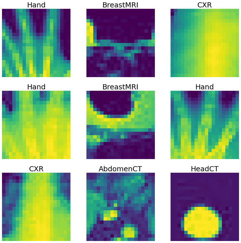
視覚化して確認するためにデータセットから画像をランダムにピックアップする
%matplotlib inline
fig, axes = plt.subplots(3, 3, figsize=(15, 15), facecolor="white")
for i, k in enumerate(np.random.randint(len(train_ds), size=9)):
    data = train_ds[k]
    im, title = data["image"], data["class_name"]
    ax = axes[i // 3, i % 3]
    im_show = ax.imshow(im[0])
    ax.set_title(title, fontsize=25)
    ax.axis("off")
損失関数とネットワークを定義する
device = "cuda" if torch.cuda.is_available() else "cpu"
loss_function = torch.nn.CrossEntropyLoss()
auc_metric = ROCAUCMetric()


def get_new_net():
    return DenseNet(
        spatial_dims=2,
        in_channels=1,
        out_channels=num_classes,
        init_features=2,
        growth_rate=2,
        block_config=(2,),
    ).to(device)


model = get_new_net()
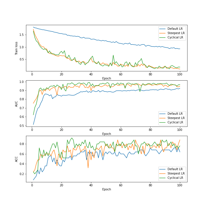
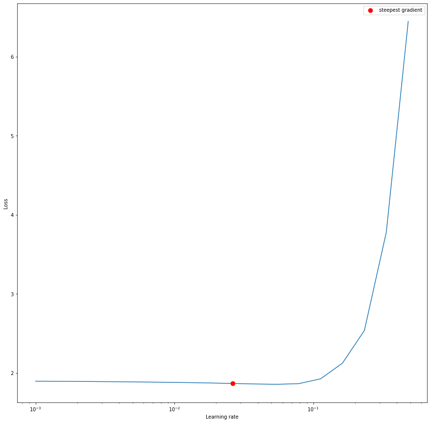
最適な学習率を推定する
MONAI の LearningRateFinder を使用して学習率の初期推定値を得ます。それは範囲 1e-5, 1e0 内にあると過程します。それが当てはまらないのであれば (プロットで気付くでしょう)、より大きな/異なるウィンドウに渡り単に再試行できるでしょう。
結果をプロットして、最も急な勾配を持つ学習率を抽出することができます。
%matplotlib inline
lower_lr, upper_lr = 1e-3, 1e-0
optimizer = torch.optim.Adam(model.parameters(), lower_lr)
lr_finder = LearningRateFinder(model, optimizer, loss_function, device=device)
lr_finder.range_test(train_loader, val_loader, end_lr=upper_lr, num_iter=20)
steepest_lr, _ = lr_finder.get_steepest_gradient()
ax = plt.subplots(1, 1, figsize=(15, 15), facecolor="white")[1]
_ = lr_finder.plot(ax=ax)
Computing optimal learning rate:  90%|█████████ | 18/20 [00:14<00:01,  1.26it/s]
Stopping early, the loss has diverged
Resetting model and optimizer
ライブ・プロッティング
この関数は、プロットが総ての反復で更新されるような、range/trange 回りの単なるラッパーです。
def plot_range(data, wrapped_generator):
    plt.ion()
    for q in data.values():
        for d in q.values():
            if isinstance(d, dict):
                ax = d["line"].axes
                ax.legend()
                fig = ax.get_figure()
    fig.show()

    for i in wrapped_generator:
        yield i
        for q in data.values():
            for d in q.values():
                if isinstance(d, dict):
                    d["line"].set_data(d["x"], d["y"])
                    ax = d["line"].axes
                    ax.legend()
                    ax.relim()
                    ax.autoscale_view()
        fig.canvas.draw()
訓練
訓練は vanilla ループとは少し違って見えますが、これは様々な学習率手法 (標準、最急 (= steepest) と周期的) の各々に渡りループし、その結果それらは同時に更新できるからです。
def get_model_optimizer_scheduler(d):
    d["model"] = get_new_net()

    if "lr_lims" in d:
        d["optimizer"] = torch.optim.Adam(
            d["model"].parameters(), d["lr_lims"][0]
        )
        d["scheduler"] = torch.optim.lr_scheduler.CyclicLR(
            d["optimizer"],
            base_lr=d["lr_lims"][0],
            max_lr=d["lr_lims"][1],
            step_size_up=d["step"],
            cycle_momentum=False,
        )
    elif "lr_lim" in d:
        d["optimizer"] = torch.optim.Adam(d["model"].parameters(), d["lr_lim"])
    else:
        d["optimizer"] = torch.optim.Adam(d["model"].parameters())


def train(max_epochs, axes, data):
    for d in data.keys():
        get_model_optimizer_scheduler(data[d])

        for q, i in enumerate(["train", "auc", "acc"]):
            data[d][i] = {"x": [], "y": []}
            (data[d][i]["line"],) = axes[q].plot(
                data[d][i]["x"], data[d][i]["y"], label=d
            )

        val_interval = 1

    for epoch in plot_range(data, trange(max_epochs)):

        for d in data.keys():
            data[d]["epoch_loss"] = 0
        for batch_data in train_loader:
            inputs = batch_data["image"].to(device)
            labels = batch_data["label"].to(device)

            for d in data.keys():
                data[d]["optimizer"].zero_grad()
                outputs = data[d]["model"](inputs)
                loss = loss_function(outputs, labels)
                loss.backward()
                data[d]["optimizer"].step()
                if "scheduler" in data[d]:
                    data[d]["scheduler"].step()
                data[d]["epoch_loss"] += loss.item()
        for d in data.keys():
            data[d]["epoch_loss"] /= len(train_loader)
            data[d]["train"]["x"].append(epoch + 1)
            data[d]["train"]["y"].append(data[d]["epoch_loss"])

        if (epoch + 1) % val_interval == 0:
            with eval_mode(*[data[d]["model"] for d in data.keys()]):
                for d in data:
                    data[d]["y_pred"] = torch.tensor(
                        [], dtype=torch.float32, device=device
                    )
                y = torch.tensor([], dtype=torch.long, device=device)
                for val_data in val_loader:
                    val_images = val_data["image"].to(device)
                    val_labels = val_data["label"].to(device)
                    for d in data:
                        data[d]["y_pred"] = torch.cat(
                            [data[d]["y_pred"], data[d]["model"](val_images)],
                            dim=0,
                        )
                    y = torch.cat([y, val_labels], dim=0)

                for d in data:
                    y_onehot = [y_trans(i) for i in decollate_batch(y)]
                    y_pred_act = [y_pred_trans(i) for i in decollate_batch(data[d]["y_pred"])]
                    auc_metric(y_pred_act, y_onehot)
                    auc_result = auc_metric.aggregate()
                    auc_metric.reset()
                    del y_pred_act, y_onehot
                    data[d]["auc"]["x"].append(epoch + 1)
                    data[d]["auc"]["y"].append(auc_result)

                    acc_value = torch.eq(data[d]["y_pred"].argmax(dim=1), y)
                    acc_metric = acc_value.sum().item() / len(acc_value)
                    data[d]["acc"]["x"].append(epoch + 1)
                    data[d]["acc"]["y"].append(acc_metric)
%matplotlib notebook
fig, axes = plt.subplots(3, 1, figsize=(10, 10), facecolor="white")
for ax in axes:
    ax.set_xlabel("Epoch")
axes[0].set_ylabel("Train loss")
axes[1].set_ylabel("AUC")
axes[2].set_ylabel("ACC")

# In the paper referenced at the top of this notebook, a step
# size of 8 times the number of iterations per epoch is suggested.
step_size = 8 * len(train_loader)

max_epochs = 100
data = {}
data["Default LR"] = {}
data["Steepest LR"] = {"lr_lim": steepest_lr}
data["Cyclical LR"] = {
    "lr_lims": (0.8 * steepest_lr, 1.2 * steepest_lr),
    "step": step_size,
}

train(max_epochs, axes, data)
100%|██████████| 100/100 [03:11<00:00, 1.91s/it]
結び
当然のことながら、Steepest LR と Cyclical LR の両方はデフォルト LR よりも損失関数の迅速な収束を示します。
この例では Steepest LR と Cyclical LR の間に大きな違いはありません。より複雑な最適化問題では大きな違いが現れるかもしれませんが、ステップサイズ、そして下限と上限の周期的制限を自由に試してください。
データディレクトリのクリーンアップ
一時ディレクトリが使用された場合にはディレクトリを削除します。
if directory is None:
    shutil.rmtree(root_dir)
以上
MONAI 0.7 : tutorials : モジュール – 層単位の学習率設定
MONAI 0.7 : tutorials : モジュール – 層単位の学習率設定 (翻訳/解説)
翻訳 : (株)クラスキャット セールスインフォメーション
作成日時 : 10/12/2021 (0.7.0)
* 本ページは、MONAI の以下のドキュメントを翻訳した上で適宜、補足説明したものです:
* サンプルコードの動作確認はしておりますが、必要な場合には適宜、追加改変しています。
* ご自由にリンクを張って頂いてかまいませんが、sales-info@classcat.com までご一報いただけると嬉しいです。
- 人工知能研究開発支援
- 人工知能研修サービス(経営者層向けオンサイト研修)
- テクニカルコンサルティングサービス
- 実証実験(プロトタイプ構築)
- アプリケーションへの実装
- 人工知能研修サービス
- PoC(概念実証)を失敗させないための支援
- テレワーク & オンライン授業を支援
- お住まいの地域に関係なく Web ブラウザからご参加頂けます。事前登録 が必要ですのでご注意ください。
- ウェビナー運用には弊社製品「ClassCat® Webinar」を利用しています。
◆ お問合せ : 本件に関するお問い合わせ先は下記までお願いいたします。
| 株式会社クラスキャット セールス・マーケティング本部 セールス・インフォメーション |
| E-Mail:sales-info@classcat.com ; WebSite: https://www.classcat.com/ ; Facebook |
MONAI 0.7 : tutorials : モジュール – 層単位の学習率設定
このノートブックは、想定されるネットワーク層を選択あるいはフィルタリングしてカスタマイズされた学習率の値を設定する方法を実演します。
このチュートリアルでは、転移学習のためにネットワーク層を選択またはフィルタリングして特定の学習率を簡単に設定する方法を紹介します。MONAI はこの要件を達成するためのユティリティ関数を提供します : 例えば、generate_param_groups です :
net = Unet(spatial_dims=3, in_channels=1, out_channels=3, channels=[2, 2, 2], strides=[1, 1, 1])
print(net)  # print out network components to select expected items
print(net.named_parameters())  # print out all the named parameters to filter out expected items
params = generate_param_groups(
    network=net,
    layer_matches=[lambda x: x.model[0], lambda x: "2.0.conv" in x[0]],
    match_types=["select", "filter"],
    lr_values=[1e-2, 1e-3],
)
optimizer = torch.optim.Adam(params, 1e-4)
環境のセットアップ
!python -c "import monai" || pip install -q "monai-weekly[pillow, ignite, tqdm]"
!python -c "import matplotlib" || pip install -q matplotlib
%matplotlib inline
from monai.transforms import (
    AddChanneld,
    Compose,
    LoadImaged,
    ScaleIntensityd,
    EnsureTyped,
)
from monai.optimizers import generate_param_groups
from monai.networks.nets import DenseNet121
from monai.inferers import SimpleInferer
from monai.handlers import StatsHandler, from_engine
from monai.engines import SupervisedTrainer
from monai.data import DataLoader
from monai.config import print_config
from monai.apps import MedNISTDataset
import torch
import matplotlib.pyplot as plt
from ignite.engine import Engine, Events
from ignite.metrics import Accuracy
import tempfile
import sys
import shutil
import os
import logging
インポートのセットアップ
# Copyright 2020 MONAI Consortium
# Licensed under the Apache License, Version 2.0 (the "License");
# you may not use this file except in compliance with the License.
# You may obtain a copy of the License at
#     http://www.apache.org/licenses/LICENSE-2.0
# Unless required by applicable law or agreed to in writing, software
# distributed under the License is distributed on an "AS IS" BASIS,
# WITHOUT WARRANTIES OR CONDITIONS OF ANY KIND, either express or implied.
# See the License for the specific language governing permissions and
# limitations under the License.


print_config()
MONAI version: 0.6.0rc1+23.gc6793fd0
Numpy version: 1.20.3
Pytorch version: 1.9.0a0+c3d40fd
MONAI flags: HAS_EXT = True, USE_COMPILED = False
MONAI rev id: c6793fd0f316a448778d0047664aaf8c1895fe1c

Optional dependencies:
Pytorch Ignite version: 0.4.5
Nibabel version: 3.2.1
scikit-image version: 0.15.0
Pillow version: 7.0.0
Tensorboard version: 2.5.0
gdown version: 3.13.0
TorchVision version: 0.10.0a0
ITK version: 5.1.2
tqdm version: 4.53.0
lmdb version: 1.2.1
psutil version: 5.8.0
pandas version: 1.1.4
einops version: 0.3.0

For details about installing the optional dependencies, please visit:
    https://docs.monai.io/en/latest/installation.html#installing-the-recommended-dependencies
データディレクトリのセットアップ
MONAI_DATA_DIRECTORY 環境変数でディレクトリを指定できます。これは結果をセーブしてダウンロードを再利用することを可能にします。指定されない場合、一時ディレクトリが使用されます。
directory = os.environ.get("MONAI_DATA_DIRECTORY")
root_dir = tempfile.mkdtemp() if directory is None else directory
print(root_dir)
ロギングのセットアップ
logging.basicConfig(stream=sys.stdout, level=logging.INFO)
MedNISTDataset とワークフローによる訓練実験の作成
MedMNIST データセットは TCIA, RSNA Bone Age チャレンジ と NIH Chest X-ray データセット からの様々なセットから集められました。
前処理変換のセットアップ
transform = Compose(
    [
        LoadImaged(keys="image"),
        AddChanneld(keys="image"),
        ScaleIntensityd(keys="image"),
        EnsureTyped(keys="image"),
    ]
)
訓練のために MedNISTDataset を作成する
MedNISTDataset は MONAI CacheDataset から継承してデータセットを自動的にダウンロードして展開するための豊富なパラメータを提供し、そしてキャッシュメカニズムを持つ通常の PyTorch データセットとして動作します。
train_ds = MedNISTDataset(
    root_dir=root_dir, transform=transform, section="training", download=True)
# the dataset can work seamlessly with the pytorch native dataset loader,
# but using monai.data.DataLoader has additional benefits of mutli-process
# random seeds handling, and the customized collate functions
train_loader = DataLoader(train_ds, batch_size=300,
                          shuffle=True, num_workers=10)
視覚化して確認するために MedNISTDataset から画像をピックアップする
plt.subplots(3, 3, figsize=(8, 8))
for i in range(9):
    plt.subplot(3, 3, i + 1)
    plt.imshow(train_ds[i * 5000]["image"][0].detach().cpu(), cmap="gray")
plt.tight_layout()
plt.show()
訓練コンポーネントを作成する – デバイス、ネットワーク、損失関数
device = torch.device("cuda:0" if torch.cuda.is_available() else "cpu")
net = DenseNet121(pretrained=True, progress=False,
                  spatial_dims=2, in_channels=1, out_channels=6).to(device)
loss = torch.nn.CrossEntropyLoss()
層のために異なる学習率の値を設定する
DenseNet121 の層についてはこのノートブックの最後の appendix を参照してください。
- 選択された class_layers ブロックのために LR=1e-3 を設定する。
- 層名に conv.weight が含まれるようなフィルタに基づく畳込み層のために LR=1e-4 を設定する。
- 他の層については LR=1e-5 。
params = generate_param_groups(
    network=net,
    layer_matches=[lambda x: x.class_layers, lambda x: "conv.weight" in x[0]],
    match_types=["select", "filter"],
    lr_values=[1e-3, 1e-4],
)
パラメータ・グループに基づいて optimizer を定義する
opt = torch.optim.Adam(params, 1e-5)
最も簡単な訓練ワークフローを定義して実行する
訓練ワークフローを素早くセットアップするために MONAI SupervisedTrainer ハンドラを使用します。
trainer = SupervisedTrainer(
    device=device,
    max_epochs=5,
    train_data_loader=train_loader,
    network=net,
    optimizer=opt,
    loss_function=loss,
    inferer=SimpleInferer(),
    key_train_metric={
        "train_acc": Accuracy(
            output_transform=from_engine(["pred", "label"]))
    },
    train_handlers=StatsHandler(
        tag_name="train_loss", output_transform=from_engine(["loss"], first=True)),
)
実行時に LR を調整するために ignite ハンドラを定義する
class LrScheduler:
    def attach(self, engine: Engine) -> None:
        engine.add_event_handler(Events.EPOCH_COMPLETED, self)

    def __call__(self, engine: Engine) -> None:
        for i, param_group in enumerate(engine.optimizer.param_groups):
            if i == 0:
                param_group["lr"] *= 0.1
            elif i == 1:
                param_group["lr"] *= 0.5

        print("LR values of 3 parameter groups: ", [
              g["lr"] for g in engine.optimizer.param_groups])


LrScheduler().attach(trainer)
訓練を実行する
trainer.run()
データディレクトリのクリーンアップ
一時ディレクトリを使用した場合ディレクトリを削除します。
if directory is None:
    shutil.rmtree(root_dir)
Appendix: DenseNet 121 ネットワークの層
print(net)
DenseNet121(
(features): Sequential(
(conv0): Conv2d(1, 64, kernel_size=(7, 7), stride=(2, 2), padding=(3, 3), bias=False)
(norm0): BatchNorm2d(64, eps=1e-05, momentum=0.1, affine=True, track_running_stats=True)
(relu0): ReLU(inplace=True)
(pool0): MaxPool2d(kernel_size=3, stride=2, padding=1, dilation=1, ceil_mode=False)
(denseblock1): _DenseBlock(
(denselayer1): _DenseLayer(
(layers): Sequential(
(norm1): BatchNorm2d(64, eps=1e-05, momentum=0.1, affine=True, track_running_stats=True)
(relu1): ReLU(inplace=True)
(conv1): Conv2d(64, 128, kernel_size=(1, 1), stride=(1, 1), bias=False)
(norm2): BatchNorm2d(128, eps=1e-05, momentum=0.1, affine=True, track_running_stats=True)
(relu2): ReLU(inplace=True)
(conv2): Conv2d(128, 32, kernel_size=(3, 3), stride=(1, 1), padding=(1, 1), bias=False)
)
)
(denselayer2): _DenseLayer(
(layers): Sequential(
(norm1): BatchNorm2d(96, eps=1e-05, momentum=0.1, affine=True, track_running_stats=True)
(relu1): ReLU(inplace=True)
(conv1): Conv2d(96, 128, kernel_size=(1, 1), stride=(1, 1), bias=False)
(norm2): BatchNorm2d(128, eps=1e-05, momentum=0.1, affine=True, track_running_stats=True)
(relu2): ReLU(inplace=True)
(conv2): Conv2d(128, 32, kernel_size=(3, 3), stride=(1, 1), padding=(1, 1), bias=False)
)
)
(denselayer3): _DenseLayer(
(layers): Sequential(
(norm1): BatchNorm2d(128, eps=1e-05, momentum=0.1, affine=True, track_running_stats=True)
(relu1): ReLU(inplace=True)
(conv1): Conv2d(128, 128, kernel_size=(1, 1), stride=(1, 1), bias=False)
(norm2): BatchNorm2d(128, eps=1e-05, momentum=0.1, affine=True, track_running_stats=True)
(relu2): ReLU(inplace=True)
(conv2): Conv2d(128, 32, kernel_size=(3, 3), stride=(1, 1), padding=(1, 1), bias=False)
)
)
(denselayer4): _DenseLayer(
(layers): Sequential(
(norm1): BatchNorm2d(160, eps=1e-05, momentum=0.1, affine=True, track_running_stats=True)
(relu1): ReLU(inplace=True)
(conv1): Conv2d(160, 128, kernel_size=(1, 1), stride=(1, 1), bias=False)
(norm2): BatchNorm2d(128, eps=1e-05, momentum=0.1, affine=True, track_running_stats=True)
(relu2): ReLU(inplace=True)
(conv2): Conv2d(128, 32, kernel_size=(3, 3), stride=(1, 1), padding=(1, 1), bias=False)
)
)
(denselayer5): _DenseLayer(
(layers): Sequential(
(norm1): BatchNorm2d(192, eps=1e-05, momentum=0.1, affine=True, track_running_stats=True)
(relu1): ReLU(inplace=True)
(conv1): Conv2d(192, 128, kernel_size=(1, 1), stride=(1, 1), bias=False)
(norm2): BatchNorm2d(128, eps=1e-05, momentum=0.1, affine=True, track_running_stats=True)
(relu2): ReLU(inplace=True)
(conv2): Conv2d(128, 32, kernel_size=(3, 3), stride=(1, 1), padding=(1, 1), bias=False)
)
)
(denselayer6): _DenseLayer(
(layers): Sequential(
(norm1): BatchNorm2d(224, eps=1e-05, momentum=0.1, affine=True, track_running_stats=True)
(relu1): ReLU(inplace=True)
(conv1): Conv2d(224, 128, kernel_size=(1, 1), stride=(1, 1), bias=False)
(norm2): BatchNorm2d(128, eps=1e-05, momentum=0.1, affine=True, track_running_stats=True)
(relu2): ReLU(inplace=True)
(conv2): Conv2d(128, 32, kernel_size=(3, 3), stride=(1, 1), padding=(1, 1), bias=False)
)
)
)
(transition1): _Transition(
(norm): BatchNorm2d(256, eps=1e-05, momentum=0.1, affine=True, track_running_stats=True)
(relu): ReLU(inplace=True)
(conv): Conv2d(256, 128, kernel_size=(1, 1), stride=(1, 1), bias=False)
(pool): AvgPool2d(kernel_size=2, stride=2, padding=0)
)
(denseblock2): _DenseBlock(
(denselayer1): _DenseLayer(
(layers): Sequential(
(norm1): BatchNorm2d(128, eps=1e-05, momentum=0.1, affine=True, track_running_stats=True)
(relu1): ReLU(inplace=True)
(conv1): Conv2d(128, 128, kernel_size=(1, 1), stride=(1, 1), bias=False)
(norm2): BatchNorm2d(128, eps=1e-05, momentum=0.1, affine=True, track_running_stats=True)
(relu2): ReLU(inplace=True)
(conv2): Conv2d(128, 32, kernel_size=(3, 3), stride=(1, 1), padding=(1, 1), bias=False)
)
)
(denselayer2): _DenseLayer(
(layers): Sequential(
(norm1): BatchNorm2d(160, eps=1e-05, momentum=0.1, affine=True, track_running_stats=True)
(relu1): ReLU(inplace=True)
(conv1): Conv2d(160, 128, kernel_size=(1, 1), stride=(1, 1), bias=False)
(norm2): BatchNorm2d(128, eps=1e-05, momentum=0.1, affine=True, track_running_stats=True)
(relu2): ReLU(inplace=True)
(conv2): Conv2d(128, 32, kernel_size=(3, 3), stride=(1, 1), padding=(1, 1), bias=False)
)
)
(denselayer3): _DenseLayer(
(layers): Sequential(
(norm1): BatchNorm2d(192, eps=1e-05, momentum=0.1, affine=True, track_running_stats=True)
(relu1): ReLU(inplace=True)
(conv1): Conv2d(192, 128, kernel_size=(1, 1), stride=(1, 1), bias=False)
(norm2): BatchNorm2d(128, eps=1e-05, momentum=0.1, affine=True, track_running_stats=True)
(relu2): ReLU(inplace=True)
(conv2): Conv2d(128, 32, kernel_size=(3, 3), stride=(1, 1), padding=(1, 1), bias=False)
)
)
(denselayer4): _DenseLayer(
(layers): Sequential(
(norm1): BatchNorm2d(224, eps=1e-05, momentum=0.1, affine=True, track_running_stats=True)
(relu1): ReLU(inplace=True)
(conv1): Conv2d(224, 128, kernel_size=(1, 1), stride=(1, 1), bias=False)
(norm2): BatchNorm2d(128, eps=1e-05, momentum=0.1, affine=True, track_running_stats=True)
(relu2): ReLU(inplace=True)
(conv2): Conv2d(128, 32, kernel_size=(3, 3), stride=(1, 1), padding=(1, 1), bias=False)
)
)
(denselayer5): _DenseLayer(
(layers): Sequential(
(norm1): BatchNorm2d(256, eps=1e-05, momentum=0.1, affine=True, track_running_stats=True)
(relu1): ReLU(inplace=True)
(conv1): Conv2d(256, 128, kernel_size=(1, 1), stride=(1, 1), bias=False)
(norm2): BatchNorm2d(128, eps=1e-05, momentum=0.1, affine=True, track_running_stats=True)
(relu2): ReLU(inplace=True)
(conv2): Conv2d(128, 32, kernel_size=(3, 3), stride=(1, 1), padding=(1, 1), bias=False)
)
)
(denselayer6): _DenseLayer(
(layers): Sequential(
(norm1): BatchNorm2d(288, eps=1e-05, momentum=0.1, affine=True, track_running_stats=True)
(relu1): ReLU(inplace=True)
(conv1): Conv2d(288, 128, kernel_size=(1, 1), stride=(1, 1), bias=False)
(norm2): BatchNorm2d(128, eps=1e-05, momentum=0.1, affine=True, track_running_stats=True)
(relu2): ReLU(inplace=True)
(conv2): Conv2d(128, 32, kernel_size=(3, 3), stride=(1, 1), padding=(1, 1), bias=False)
)
)
(denselayer7): _DenseLayer(
(layers): Sequential(
(norm1): BatchNorm2d(320, eps=1e-05, momentum=0.1, affine=True, track_running_stats=True)
(relu1): ReLU(inplace=True)
(conv1): Conv2d(320, 128, kernel_size=(1, 1), stride=(1, 1), bias=False)
(norm2): BatchNorm2d(128, eps=1e-05, momentum=0.1, affine=True, track_running_stats=True)
(relu2): ReLU(inplace=True)
(conv2): Conv2d(128, 32, kernel_size=(3, 3), stride=(1, 1), padding=(1, 1), bias=False)
)
)
(denselayer8): _DenseLayer(
(layers): Sequential(
(norm1): BatchNorm2d(352, eps=1e-05, momentum=0.1, affine=True, track_running_stats=True)
(relu1): ReLU(inplace=True)
(conv1): Conv2d(352, 128, kernel_size=(1, 1), stride=(1, 1), bias=False)
(norm2): BatchNorm2d(128, eps=1e-05, momentum=0.1, affine=True, track_running_stats=True)
(relu2): ReLU(inplace=True)
(conv2): Conv2d(128, 32, kernel_size=(3, 3), stride=(1, 1), padding=(1, 1), bias=False)
)
)
(denselayer9): _DenseLayer(
(layers): Sequential(
(norm1): BatchNorm2d(384, eps=1e-05, momentum=0.1, affine=True, track_running_stats=True)
(relu1): ReLU(inplace=True)
(conv1): Conv2d(384, 128, kernel_size=(1, 1), stride=(1, 1), bias=False)
(norm2): BatchNorm2d(128, eps=1e-05, momentum=0.1, affine=True, track_running_stats=True)
(relu2): ReLU(inplace=True)
(conv2): Conv2d(128, 32, kernel_size=(3, 3), stride=(1, 1), padding=(1, 1), bias=False)
)
)
(denselayer10): _DenseLayer(
(layers): Sequential(
(norm1): BatchNorm2d(416, eps=1e-05, momentum=0.1, affine=True, track_running_stats=True)
(relu1): ReLU(inplace=True)
(conv1): Conv2d(416, 128, kernel_size=(1, 1), stride=(1, 1), bias=False)
(norm2): BatchNorm2d(128, eps=1e-05, momentum=0.1, affine=True, track_running_stats=True)
(relu2): ReLU(inplace=True)
(conv2): Conv2d(128, 32, kernel_size=(3, 3), stride=(1, 1), padding=(1, 1), bias=False)
)
)
(denselayer11): _DenseLayer(
(layers): Sequential(
(norm1): BatchNorm2d(448, eps=1e-05, momentum=0.1, affine=True, track_running_stats=True)
(relu1): ReLU(inplace=True)
(conv1): Conv2d(448, 128, kernel_size=(1, 1), stride=(1, 1), bias=False)
(norm2): BatchNorm2d(128, eps=1e-05, momentum=0.1, affine=True, track_running_stats=True)
(relu2): ReLU(inplace=True)
(conv2): Conv2d(128, 32, kernel_size=(3, 3), stride=(1, 1), padding=(1, 1), bias=False)
)
)
(denselayer12): _DenseLayer(
(layers): Sequential(
(norm1): BatchNorm2d(480, eps=1e-05, momentum=0.1, affine=True, track_running_stats=True)
(relu1): ReLU(inplace=True)
(conv1): Conv2d(480, 128, kernel_size=(1, 1), stride=(1, 1), bias=False)
(norm2): BatchNorm2d(128, eps=1e-05, momentum=0.1, affine=True, track_running_stats=True)
(relu2): ReLU(inplace=True)
(conv2): Conv2d(128, 32, kernel_size=(3, 3), stride=(1, 1), padding=(1, 1), bias=False)
)
)
)
(transition2): _Transition(
(norm): BatchNorm2d(512, eps=1e-05, momentum=0.1, affine=True, track_running_stats=True)
(relu): ReLU(inplace=True)
(conv): Conv2d(512, 256, kernel_size=(1, 1), stride=(1, 1), bias=False)
(pool): AvgPool2d(kernel_size=2, stride=2, padding=0)
)
(denseblock3): _DenseBlock(
(denselayer1): _DenseLayer(
(layers): Sequential(
(norm1): BatchNorm2d(256, eps=1e-05, momentum=0.1, affine=True, track_running_stats=True)
(relu1): ReLU(inplace=True)
(conv1): Conv2d(256, 128, kernel_size=(1, 1), stride=(1, 1), bias=False)
(norm2): BatchNorm2d(128, eps=1e-05, momentum=0.1, affine=True, track_running_stats=True)
(relu2): ReLU(inplace=True)
(conv2): Conv2d(128, 32, kernel_size=(3, 3), stride=(1, 1), padding=(1, 1), bias=False)
)
)
(denselayer2): _DenseLayer(
(layers): Sequential(
(norm1): BatchNorm2d(288, eps=1e-05, momentum=0.1, affine=True, track_running_stats=True)
(relu1): ReLU(inplace=True)
(conv1): Conv2d(288, 128, kernel_size=(1, 1), stride=(1, 1), bias=False)
(norm2): BatchNorm2d(128, eps=1e-05, momentum=0.1, affine=True, track_running_stats=True)
(relu2): ReLU(inplace=True)
(conv2): Conv2d(128, 32, kernel_size=(3, 3), stride=(1, 1), padding=(1, 1), bias=False)
)
)
(denselayer3): _DenseLayer(
(layers): Sequential(
(norm1): BatchNorm2d(320, eps=1e-05, momentum=0.1, affine=True, track_running_stats=True)
(relu1): ReLU(inplace=True)
(conv1): Conv2d(320, 128, kernel_size=(1, 1), stride=(1, 1), bias=False)
(norm2): BatchNorm2d(128, eps=1e-05, momentum=0.1, affine=True, track_running_stats=True)
(relu2): ReLU(inplace=True)
(conv2): Conv2d(128, 32, kernel_size=(3, 3), stride=(1, 1), padding=(1, 1), bias=False)
)
)
(denselayer4): _DenseLayer(
(layers): Sequential(
(norm1): BatchNorm2d(352, eps=1e-05, momentum=0.1, affine=True, track_running_stats=True)
(relu1): ReLU(inplace=True)
(conv1): Conv2d(352, 128, kernel_size=(1, 1), stride=(1, 1), bias=False)
(norm2): BatchNorm2d(128, eps=1e-05, momentum=0.1, affine=True, track_running_stats=True)
(relu2): ReLU(inplace=True)
(conv2): Conv2d(128, 32, kernel_size=(3, 3), stride=(1, 1), padding=(1, 1), bias=False)
)
)
(denselayer5): _DenseLayer(
(layers): Sequential(
(norm1): BatchNorm2d(384, eps=1e-05, momentum=0.1, affine=True, track_running_stats=True)
(relu1): ReLU(inplace=True)
(conv1): Conv2d(384, 128, kernel_size=(1, 1), stride=(1, 1), bias=False)
(norm2): BatchNorm2d(128, eps=1e-05, momentum=0.1, affine=True, track_running_stats=True)
(relu2): ReLU(inplace=True)
(conv2): Conv2d(128, 32, kernel_size=(3, 3), stride=(1, 1), padding=(1, 1), bias=False)
)
)
(denselayer6): _DenseLayer(
(layers): Sequential(
(norm1): BatchNorm2d(416, eps=1e-05, momentum=0.1, affine=True, track_running_stats=True)
(relu1): ReLU(inplace=True)
(conv1): Conv2d(416, 128, kernel_size=(1, 1), stride=(1, 1), bias=False)
(norm2): BatchNorm2d(128, eps=1e-05, momentum=0.1, affine=True, track_running_stats=True)
(relu2): ReLU(inplace=True)
(conv2): Conv2d(128, 32, kernel_size=(3, 3), stride=(1, 1), padding=(1, 1), bias=False)
)
)
(denselayer7): _DenseLayer(
(layers): Sequential(
(norm1): BatchNorm2d(448, eps=1e-05, momentum=0.1, affine=True, track_running_stats=True)
(relu1): ReLU(inplace=True)
(conv1): Conv2d(448, 128, kernel_size=(1, 1), stride=(1, 1), bias=False)
(norm2): BatchNorm2d(128, eps=1e-05, momentum=0.1, affine=True, track_running_stats=True)
(relu2): ReLU(inplace=True)
(conv2): Conv2d(128, 32, kernel_size=(3, 3), stride=(1, 1), padding=(1, 1), bias=False)
)
)
(denselayer8): _DenseLayer(
(layers): Sequential(
(norm1): BatchNorm2d(480, eps=1e-05, momentum=0.1, affine=True, track_running_stats=True)
(relu1): ReLU(inplace=True)
(conv1): Conv2d(480, 128, kernel_size=(1, 1), stride=(1, 1), bias=False)
(norm2): BatchNorm2d(128, eps=1e-05, momentum=0.1, affine=True, track_running_stats=True)
(relu2): ReLU(inplace=True)
(conv2): Conv2d(128, 32, kernel_size=(3, 3), stride=(1, 1), padding=(1, 1), bias=False)
)
)
(denselayer9): _DenseLayer(
(layers): Sequential(
(norm1): BatchNorm2d(512, eps=1e-05, momentum=0.1, affine=True, track_running_stats=True)
(relu1): ReLU(inplace=True)
(conv1): Conv2d(512, 128, kernel_size=(1, 1), stride=(1, 1), bias=False)
(norm2): BatchNorm2d(128, eps=1e-05, momentum=0.1, affine=True, track_running_stats=True)
(relu2): ReLU(inplace=True)
(conv2): Conv2d(128, 32, kernel_size=(3, 3), stride=(1, 1), padding=(1, 1), bias=False)
)
)
(denselayer10): _DenseLayer(
(layers): Sequential(
(norm1): BatchNorm2d(544, eps=1e-05, momentum=0.1, affine=True, track_running_stats=True)
(relu1): ReLU(inplace=True)
(conv1): Conv2d(544, 128, kernel_size=(1, 1), stride=(1, 1), bias=False)
(norm2): BatchNorm2d(128, eps=1e-05, momentum=0.1, affine=True, track_running_stats=True)
(relu2): ReLU(inplace=True)
(conv2): Conv2d(128, 32, kernel_size=(3, 3), stride=(1, 1), padding=(1, 1), bias=False)
)
)
(denselayer11): _DenseLayer(
(layers): Sequential(
(norm1): BatchNorm2d(576, eps=1e-05, momentum=0.1, affine=True, track_running_stats=True)
(relu1): ReLU(inplace=True)
(conv1): Conv2d(576, 128, kernel_size=(1, 1), stride=(1, 1), bias=False)
(norm2): BatchNorm2d(128, eps=1e-05, momentum=0.1, affine=True, track_running_stats=True)
(relu2): ReLU(inplace=True)
(conv2): Conv2d(128, 32, kernel_size=(3, 3), stride=(1, 1), padding=(1, 1), bias=False)
)
)
(denselayer12): _DenseLayer(
(layers): Sequential(
(norm1): BatchNorm2d(608, eps=1e-05, momentum=0.1, affine=True, track_running_stats=True)
(relu1): ReLU(inplace=True)
(conv1): Conv2d(608, 128, kernel_size=(1, 1), stride=(1, 1), bias=False)
(norm2): BatchNorm2d(128, eps=1e-05, momentum=0.1, affine=True, track_running_stats=True)
(relu2): ReLU(inplace=True)
(conv2): Conv2d(128, 32, kernel_size=(3, 3), stride=(1, 1), padding=(1, 1), bias=False)
)
)
(denselayer13): _DenseLayer(
(layers): Sequential(
(norm1): BatchNorm2d(640, eps=1e-05, momentum=0.1, affine=True, track_running_stats=True)
(relu1): ReLU(inplace=True)
(conv1): Conv2d(640, 128, kernel_size=(1, 1), stride=(1, 1), bias=False)
(norm2): BatchNorm2d(128, eps=1e-05, momentum=0.1, affine=True, track_running_stats=True)
(relu2): ReLU(inplace=True)
(conv2): Conv2d(128, 32, kernel_size=(3, 3), stride=(1, 1), padding=(1, 1), bias=False)
)
)
(denselayer14): _DenseLayer(
(layers): Sequential(
(norm1): BatchNorm2d(672, eps=1e-05, momentum=0.1, affine=True, track_running_stats=True)
(relu1): ReLU(inplace=True)
(conv1): Conv2d(672, 128, kernel_size=(1, 1), stride=(1, 1), bias=False)
(norm2): BatchNorm2d(128, eps=1e-05, momentum=0.1, affine=True, track_running_stats=True)
(relu2): ReLU(inplace=True)
(conv2): Conv2d(128, 32, kernel_size=(3, 3), stride=(1, 1), padding=(1, 1), bias=False)
)
)
(denselayer15): _DenseLayer(
(layers): Sequential(
(norm1): BatchNorm2d(704, eps=1e-05, momentum=0.1, affine=True, track_running_stats=True)
(relu1): ReLU(inplace=True)
(conv1): Conv2d(704, 128, kernel_size=(1, 1), stride=(1, 1), bias=False)
(norm2): BatchNorm2d(128, eps=1e-05, momentum=0.1, affine=True, track_running_stats=True)
(relu2): ReLU(inplace=True)
(conv2): Conv2d(128, 32, kernel_size=(3, 3), stride=(1, 1), padding=(1, 1), bias=False)
)
)
(denselayer16): _DenseLayer(
(layers): Sequential(
(norm1): BatchNorm2d(736, eps=1e-05, momentum=0.1, affine=True, track_running_stats=True)
(relu1): ReLU(inplace=True)
(conv1): Conv2d(736, 128, kernel_size=(1, 1), stride=(1, 1), bias=False)
(norm2): BatchNorm2d(128, eps=1e-05, momentum=0.1, affine=True, track_running_stats=True)
(relu2): ReLU(inplace=True)
(conv2): Conv2d(128, 32, kernel_size=(3, 3), stride=(1, 1), padding=(1, 1), bias=False)
)
)
(denselayer17): _DenseLayer(
(layers): Sequential(
(norm1): BatchNorm2d(768, eps=1e-05, momentum=0.1, affine=True, track_running_stats=True)
(relu1): ReLU(inplace=True)
(conv1): Conv2d(768, 128, kernel_size=(1, 1), stride=(1, 1), bias=False)
(norm2): BatchNorm2d(128, eps=1e-05, momentum=0.1, affine=True, track_running_stats=True)
(relu2): ReLU(inplace=True)
(conv2): Conv2d(128, 32, kernel_size=(3, 3), stride=(1, 1), padding=(1, 1), bias=False)
)
)
(denselayer18): _DenseLayer(
(layers): Sequential(
(norm1): BatchNorm2d(800, eps=1e-05, momentum=0.1, affine=True, track_running_stats=True)
(relu1): ReLU(inplace=True)
(conv1): Conv2d(800, 128, kernel_size=(1, 1), stride=(1, 1), bias=False)
(norm2): BatchNorm2d(128, eps=1e-05, momentum=0.1, affine=True, track_running_stats=True)
(relu2): ReLU(inplace=True)
(conv2): Conv2d(128, 32, kernel_size=(3, 3), stride=(1, 1), padding=(1, 1), bias=False)
)
)
(denselayer19): _DenseLayer(
(layers): Sequential(
(norm1): BatchNorm2d(832, eps=1e-05, momentum=0.1, affine=True, track_running_stats=True)
(relu1): ReLU(inplace=True)
(conv1): Conv2d(832, 128, kernel_size=(1, 1), stride=(1, 1), bias=False)
(norm2): BatchNorm2d(128, eps=1e-05, momentum=0.1, affine=True, track_running_stats=True)
(relu2): ReLU(inplace=True)
(conv2): Conv2d(128, 32, kernel_size=(3, 3), stride=(1, 1), padding=(1, 1), bias=False)
)
)
(denselayer20): _DenseLayer(
(layers): Sequential(
(norm1): BatchNorm2d(864, eps=1e-05, momentum=0.1, affine=True, track_running_stats=True)
(relu1): ReLU(inplace=True)
(conv1): Conv2d(864, 128, kernel_size=(1, 1), stride=(1, 1), bias=False)
(norm2): BatchNorm2d(128, eps=1e-05, momentum=0.1, affine=True, track_running_stats=True)
(relu2): ReLU(inplace=True)
(conv2): Conv2d(128, 32, kernel_size=(3, 3), stride=(1, 1), padding=(1, 1), bias=False)
)
)
(denselayer21): _DenseLayer(
(layers): Sequential(
(norm1): BatchNorm2d(896, eps=1e-05, momentum=0.1, affine=True, track_running_stats=True)
(relu1): ReLU(inplace=True)
(conv1): Conv2d(896, 128, kernel_size=(1, 1), stride=(1, 1), bias=False)
(norm2): BatchNorm2d(128, eps=1e-05, momentum=0.1, affine=True, track_running_stats=True)
(relu2): ReLU(inplace=True)
(conv2): Conv2d(128, 32, kernel_size=(3, 3), stride=(1, 1), padding=(1, 1), bias=False)
)
)
(denselayer22): _DenseLayer(
(layers): Sequential(
(norm1): BatchNorm2d(928, eps=1e-05, momentum=0.1, affine=True, track_running_stats=True)
(relu1): ReLU(inplace=True)
(conv1): Conv2d(928, 128, kernel_size=(1, 1), stride=(1, 1), bias=False)
(norm2): BatchNorm2d(128, eps=1e-05, momentum=0.1, affine=True, track_running_stats=True)
(relu2): ReLU(inplace=True)
(conv2): Conv2d(128, 32, kernel_size=(3, 3), stride=(1, 1), padding=(1, 1), bias=False)
)
)
(denselayer23): _DenseLayer(
(layers): Sequential(
(norm1): BatchNorm2d(960, eps=1e-05, momentum=0.1, affine=True, track_running_stats=True)
(relu1): ReLU(inplace=True)
(conv1): Conv2d(960, 128, kernel_size=(1, 1), stride=(1, 1), bias=False)
(norm2): BatchNorm2d(128, eps=1e-05, momentum=0.1, affine=True, track_running_stats=True)
(relu2): ReLU(inplace=True)
(conv2): Conv2d(128, 32, kernel_size=(3, 3), stride=(1, 1), padding=(1, 1), bias=False)
)
)
(denselayer24): _DenseLayer(
(layers): Sequential(
(norm1): BatchNorm2d(992, eps=1e-05, momentum=0.1, affine=True, track_running_stats=True)
(relu1): ReLU(inplace=True)
(conv1): Conv2d(992, 128, kernel_size=(1, 1), stride=(1, 1), bias=False)
(norm2): BatchNorm2d(128, eps=1e-05, momentum=0.1, affine=True, track_running_stats=True)
(relu2): ReLU(inplace=True)
(conv2): Conv2d(128, 32, kernel_size=(3, 3), stride=(1, 1), padding=(1, 1), bias=False)
)
)
)
(transition3): _Transition(
(norm): BatchNorm2d(1024, eps=1e-05, momentum=0.1, affine=True, track_running_stats=True)
(relu): ReLU(inplace=True)
(conv): Conv2d(1024, 512, kernel_size=(1, 1), stride=(1, 1), bias=False)
(pool): AvgPool2d(kernel_size=2, stride=2, padding=0)
)
(denseblock4): _DenseBlock(
(denselayer1): _DenseLayer(
(layers): Sequential(
(norm1): BatchNorm2d(512, eps=1e-05, momentum=0.1, affine=True, track_running_stats=True)
(relu1): ReLU(inplace=True)
(conv1): Conv2d(512, 128, kernel_size=(1, 1), stride=(1, 1), bias=False)
(norm2): BatchNorm2d(128, eps=1e-05, momentum=0.1, affine=True, track_running_stats=True)
(relu2): ReLU(inplace=True)
(conv2): Conv2d(128, 32, kernel_size=(3, 3), stride=(1, 1), padding=(1, 1), bias=False)
)
)
(denselayer2): _DenseLayer(
(layers): Sequential(
(norm1): BatchNorm2d(544, eps=1e-05, momentum=0.1, affine=True, track_running_stats=True)
(relu1): ReLU(inplace=True)
(conv1): Conv2d(544, 128, kernel_size=(1, 1), stride=(1, 1), bias=False)
(norm2): BatchNorm2d(128, eps=1e-05, momentum=0.1, affine=True, track_running_stats=True)
(relu2): ReLU(inplace=True)
(conv2): Conv2d(128, 32, kernel_size=(3, 3), stride=(1, 1), padding=(1, 1), bias=False)
)
)
(denselayer3): _DenseLayer(
(layers): Sequential(
(norm1): BatchNorm2d(576, eps=1e-05, momentum=0.1, affine=True, track_running_stats=True)
(relu1): ReLU(inplace=True)
(conv1): Conv2d(576, 128, kernel_size=(1, 1), stride=(1, 1), bias=False)
(norm2): BatchNorm2d(128, eps=1e-05, momentum=0.1, affine=True, track_running_stats=True)
(relu2): ReLU(inplace=True)
(conv2): Conv2d(128, 32, kernel_size=(3, 3), stride=(1, 1), padding=(1, 1), bias=False)
)
)
(denselayer4): _DenseLayer(
(layers): Sequential(
(norm1): BatchNorm2d(608, eps=1e-05, momentum=0.1, affine=True, track_running_stats=True)
(relu1): ReLU(inplace=True)
(conv1): Conv2d(608, 128, kernel_size=(1, 1), stride=(1, 1), bias=False)
(norm2): BatchNorm2d(128, eps=1e-05, momentum=0.1, affine=True, track_running_stats=True)
(relu2): ReLU(inplace=True)
(conv2): Conv2d(128, 32, kernel_size=(3, 3), stride=(1, 1), padding=(1, 1), bias=False)
)
)
(denselayer5): _DenseLayer(
(layers): Sequential(
(norm1): BatchNorm2d(640, eps=1e-05, momentum=0.1, affine=True, track_running_stats=True)
(relu1): ReLU(inplace=True)
(conv1): Conv2d(640, 128, kernel_size=(1, 1), stride=(1, 1), bias=False)
(norm2): BatchNorm2d(128, eps=1e-05, momentum=0.1, affine=True, track_running_stats=True)
(relu2): ReLU(inplace=True)
(conv2): Conv2d(128, 32, kernel_size=(3, 3), stride=(1, 1), padding=(1, 1), bias=False)
)
)
(denselayer6): _DenseLayer(
(layers): Sequential(
(norm1): BatchNorm2d(672, eps=1e-05, momentum=0.1, affine=True, track_running_stats=True)
(relu1): ReLU(inplace=True)
(conv1): Conv2d(672, 128, kernel_size=(1, 1), stride=(1, 1), bias=False)
(norm2): BatchNorm2d(128, eps=1e-05, momentum=0.1, affine=True, track_running_stats=True)
(relu2): ReLU(inplace=True)
(conv2): Conv2d(128, 32, kernel_size=(3, 3), stride=(1, 1), padding=(1, 1), bias=False)
)
)
(denselayer7): _DenseLayer(
(layers): Sequential(
(norm1): BatchNorm2d(704, eps=1e-05, momentum=0.1, affine=True, track_running_stats=True)
(relu1): ReLU(inplace=True)
(conv1): Conv2d(704, 128, kernel_size=(1, 1), stride=(1, 1), bias=False)
(norm2): BatchNorm2d(128, eps=1e-05, momentum=0.1, affine=True, track_running_stats=True)
(relu2): ReLU(inplace=True)
(conv2): Conv2d(128, 32, kernel_size=(3, 3), stride=(1, 1), padding=(1, 1), bias=False)
)
)
(denselayer8): _DenseLayer(
(layers): Sequential(
(norm1): BatchNorm2d(736, eps=1e-05, momentum=0.1, affine=True, track_running_stats=True)
(relu1): ReLU(inplace=True)
(conv1): Conv2d(736, 128, kernel_size=(1, 1), stride=(1, 1), bias=False)
(norm2): BatchNorm2d(128, eps=1e-05, momentum=0.1, affine=True, track_running_stats=True)
(relu2): ReLU(inplace=True)
(conv2): Conv2d(128, 32, kernel_size=(3, 3), stride=(1, 1), padding=(1, 1), bias=False)
)
)
(denselayer9): _DenseLayer(
(layers): Sequential(
(norm1): BatchNorm2d(768, eps=1e-05, momentum=0.1, affine=True, track_running_stats=True)
(relu1): ReLU(inplace=True)
(conv1): Conv2d(768, 128, kernel_size=(1, 1), stride=(1, 1), bias=False)
(norm2): BatchNorm2d(128, eps=1e-05, momentum=0.1, affine=True, track_running_stats=True)
(relu2): ReLU(inplace=True)
(conv2): Conv2d(128, 32, kernel_size=(3, 3), stride=(1, 1), padding=(1, 1), bias=False)
)
)
(denselayer10): _DenseLayer(
(layers): Sequential(
(norm1): BatchNorm2d(800, eps=1e-05, momentum=0.1, affine=True, track_running_stats=True)
(relu1): ReLU(inplace=True)
(conv1): Conv2d(800, 128, kernel_size=(1, 1), stride=(1, 1), bias=False)
(norm2): BatchNorm2d(128, eps=1e-05, momentum=0.1, affine=True, track_running_stats=True)
(relu2): ReLU(inplace=True)
(conv2): Conv2d(128, 32, kernel_size=(3, 3), stride=(1, 1), padding=(1, 1), bias=False)
)
)
(denselayer11): _DenseLayer(
(layers): Sequential(
(norm1): BatchNorm2d(832, eps=1e-05, momentum=0.1, affine=True, track_running_stats=True)
(relu1): ReLU(inplace=True)
(conv1): Conv2d(832, 128, kernel_size=(1, 1), stride=(1, 1), bias=False)
(norm2): BatchNorm2d(128, eps=1e-05, momentum=0.1, affine=True, track_running_stats=True)
(relu2): ReLU(inplace=True)
(conv2): Conv2d(128, 32, kernel_size=(3, 3), stride=(1, 1), padding=(1, 1), bias=False)
)
)
(denselayer12): _DenseLayer(
(layers): Sequential(
(norm1): BatchNorm2d(864, eps=1e-05, momentum=0.1, affine=True, track_running_stats=True)
(relu1): ReLU(inplace=True)
(conv1): Conv2d(864, 128, kernel_size=(1, 1), stride=(1, 1), bias=False)
(norm2): BatchNorm2d(128, eps=1e-05, momentum=0.1, affine=True, track_running_stats=True)
(relu2): ReLU(inplace=True)
(conv2): Conv2d(128, 32, kernel_size=(3, 3), stride=(1, 1), padding=(1, 1), bias=False)
)
)
(denselayer13): _DenseLayer(
(layers): Sequential(
(norm1): BatchNorm2d(896, eps=1e-05, momentum=0.1, affine=True, track_running_stats=True)
(relu1): ReLU(inplace=True)
(conv1): Conv2d(896, 128, kernel_size=(1, 1), stride=(1, 1), bias=False)
(norm2): BatchNorm2d(128, eps=1e-05, momentum=0.1, affine=True, track_running_stats=True)
(relu2): ReLU(inplace=True)
(conv2): Conv2d(128, 32, kernel_size=(3, 3), stride=(1, 1), padding=(1, 1), bias=False)
)
)
(denselayer14): _DenseLayer(
(layers): Sequential(
(norm1): BatchNorm2d(928, eps=1e-05, momentum=0.1, affine=True, track_running_stats=True)
(relu1): ReLU(inplace=True)
(conv1): Conv2d(928, 128, kernel_size=(1, 1), stride=(1, 1), bias=False)
(norm2): BatchNorm2d(128, eps=1e-05, momentum=0.1, affine=True, track_running_stats=True)
(relu2): ReLU(inplace=True)
(conv2): Conv2d(128, 32, kernel_size=(3, 3), stride=(1, 1), padding=(1, 1), bias=False)
)
)
(denselayer15): _DenseLayer(
(layers): Sequential(
(norm1): BatchNorm2d(960, eps=1e-05, momentum=0.1, affine=True, track_running_stats=True)
(relu1): ReLU(inplace=True)
(conv1): Conv2d(960, 128, kernel_size=(1, 1), stride=(1, 1), bias=False)
(norm2): BatchNorm2d(128, eps=1e-05, momentum=0.1, affine=True, track_running_stats=True)
(relu2): ReLU(inplace=True)
(conv2): Conv2d(128, 32, kernel_size=(3, 3), stride=(1, 1), padding=(1, 1), bias=False)
)
)
(denselayer16): _DenseLayer(
(layers): Sequential(
(norm1): BatchNorm2d(992, eps=1e-05, momentum=0.1, affine=True, track_running_stats=True)
(relu1): ReLU(inplace=True)
(conv1): Conv2d(992, 128, kernel_size=(1, 1), stride=(1, 1), bias=False)
(norm2): BatchNorm2d(128, eps=1e-05, momentum=0.1, affine=True, track_running_stats=True)
(relu2): ReLU(inplace=True)
(conv2): Conv2d(128, 32, kernel_size=(3, 3), stride=(1, 1), padding=(1, 1), bias=False)
)
)
)
(norm5): BatchNorm2d(1024, eps=1e-05, momentum=0.1, affine=True, track_running_stats=True)
)
(class_layers): Sequential(
(relu): ReLU(inplace=True)
(pool): AdaptiveAvgPool2d(output_size=1)
(flatten): Flatten(start_dim=1, end_dim=-1)
(out): Linear(in_features=1024, out_features=6, bias=True)
)
)
以上
MONAI 0.7 : tutorials : モジュール – 2D 画像変換デモ
MONAI 0.7 : tutorials : モジュール – 2D 画像変換デモ (翻訳/解説)
翻訳 : (株)クラスキャット セールスインフォメーション
作成日時 : 10/12/2021 (0.7.0)
* 本ページは、MONAI の以下のドキュメントを翻訳した上で適宜、補足説明したものです:
* サンプルコードの動作確認はしておりますが、必要な場合には適宜、追加改変しています。
* ご自由にリンクを張って頂いてかまいませんが、sales-info@classcat.com までご一報いただけると嬉しいです。
- 人工知能研究開発支援
- 人工知能研修サービス(経営者層向けオンサイト研修)
- テクニカルコンサルティングサービス
- 実証実験(プロトタイプ構築)
- アプリケーションへの実装
- 人工知能研修サービス
- PoC(概念実証)を失敗させないための支援
- テレワーク & オンライン授業を支援
- お住まいの地域に関係なく Web ブラウザからご参加頂けます。事前登録 が必要ですのでご注意ください。
- ウェビナー運用には弊社製品「ClassCat® Webinar」を利用しています。
◆ お問合せ : 本件に関するお問い合わせ先は下記までお願いいたします。
| 株式会社クラスキャット セールス・マーケティング本部 セールス・インフォメーション |
| E-Mail:sales-info@classcat.com ; WebSite: https://www.classcat.com/ ; Facebook |
![]()
MONAI 0.7 : tutorials : モジュール – 2D 画像変換デモ
このノートブックは GlaS Contest データセット を使用して組織学 (= histology) の画像上の画像変換を実演します。
このデモは MONAI の 2D 変換を適用する方法を示します。主要な特徴は :
- ネイティブ PyTorch で実装されたランダムな elastic 変換
- pythonic な方法で設計されて実装された使いやすいインターフェイス
詳細は MONAI の wiki ページで調べてください : https://github.com/Project-MONAI/MONAI/wiki
環境のセットアップ
!python -c "import monai" || pip install -q "monai-weekly[pillow,tqdm]"
!python -c "import matplotlib" || pip install -q matplotlib
%matplotlib inline
from monai.transforms import Affine, Rand2DElastic
from monai.config import print_config
from monai.apps import download_and_extract
import torch
import PIL
import numpy as np
import matplotlib.pyplot as plt
import tempfile
import shutil
import os
インポートのセットアップ
# Copyright 2020 MONAI Consortium
# Licensed under the Apache License, Version 2.0 (the "License");
# you may not use this file except in compliance with the License.
# You may obtain a copy of the License at
#     http://www.apache.org/licenses/LICENSE-2.0
# Unless required by applicable law or agreed to in writing, software
# distributed under the License is distributed on an "AS IS" BASIS,
# WITHOUT WARRANTIES OR CONDITIONS OF ANY KIND, either express or implied.
# See the License for the specific language governing permissions and
# limitations under the License.


print_config()
MONAI version: 0.6.0+135.g3cb355bb
Numpy version: 1.21.2
Pytorch version: 1.9.0
MONAI flags: HAS_EXT = False, USE_COMPILED = False
MONAI rev id: 3cb355bb4e50702a17854cea1b817076c021c1b5

Optional dependencies:
Pytorch Ignite version: 0.4.5
Nibabel version: 3.2.1
scikit-image version: 0.18.3
Pillow version: 8.3.2
Tensorboard version: 2.6.0
gdown version: 3.13.0
TorchVision version: 0.10.0
tqdm version: 4.62.2
lmdb version: 1.2.1
psutil version: 5.8.0
pandas version: 1.3.3
einops version: 0.3.2

For details about installing the optional dependencies, please visit:
    https://docs.monai.io/en/latest/installation.html#installing-the-recommended-dependencies
データディレクトリのセットアップ
MONAI_DATA_DIRECTORY 環境変数でディレクトリを指定できます。これは結果をセーブしてダウンロードを再利用することを可能にします。指定されない場合、一時ディレクトリが使用されます。
directory = os.environ.get("MONAI_DATA_DIRECTORY")
root_dir = tempfile.mkdtemp() if directory is None else directory
print(root_dir)
/var/folders/6f/fdkl7m0x7sz3nj_t7p3ccgz00000gp/T/tmpo87g5vor
データセットのダウンロード
データセットをダウンロードして解凍します。データセットは https://warwick.ac.uk/fac/sci/dcs/research/tia/glascontest/ に由来します。
このコンペで使用されたデータセットは研究目的のみで提供されます。商用利用は許容されません。
K. Sirinukunwattana, J. P. W. Pluim, H. Chen, X Qi, P. Heng, Y. Guo, L. Wang, B. J. Matuszewski, E. Bruni, U. Sanchez, A. Böhm, O. Ronneberger, B. Ben Cheikh, D. Racoceanu, P. Kainz, M. Pfeiffer, M. Urschler, D. R. J. Snead, N. M. Rajpoot, “Gland Segmentation in Colon Histology Images: The GlaS Challenge Contest” http://arxiv.org/abs/1603.00275
K. Sirinukunwattana, D.R.J. Snead, N.M. Rajpoot, “A Stochastic Polygons Model for Glandular Structures in Colon Histology Images,” in IEEE Transactions on Medical Imaging, 2015 doi: 10.1109/TMI.2015.2433900
resource = "https://warwick.ac.uk/fac/sci/dcs/research/tia/" \
    + "glascontest/download/warwick_qu_dataset_released_2016_07_08.zip"
md5 = None

compressed_file = os.path.join(
    root_dir, "warwick_qu_dataset_released_2016_07_08.zip")
data_dir = os.path.join(root_dir, "Warwick QU Dataset (Released 2016_07_08)")
if not os.path.exists(data_dir):
    download_and_extract(resource, compressed_file, root_dir, md5)
warwick_qu_dataset_released_2016_07_08.zip: 173MB [00:20, 8.95MB/s]
Downloaded: /var/folders/6f/fdkl7m0x7sz3nj_t7p3ccgz00000gp/T/tmpo87g5vor/warwick_qu_dataset_released_2016_07_08.zip
Expected md5 is None, skip md5 check for file /var/folders/6f/fdkl7m0x7sz3nj_t7p3ccgz00000gp/T/tmpo87g5vor/warwick_qu_dataset_released_2016_07_08.zip.
Writing into directory: /var/folders/6f/fdkl7m0x7sz3nj_t7p3ccgz00000gp/T/tmpo87g5vor.
device = "cpu" if not torch.cuda.is_available() else "cuda:0"
img_name = os.path.join(data_dir, "train_22.bmp")
seg_name = os.path.join(data_dir, "train_22_anno.bmp")
im = np.array(PIL.Image.open(img_name))
seg = np.array(PIL.Image.open(seg_name))
plt.figure("check", (12, 6))
plt.subplot(1, 2, 1)
plt.title("image")
plt.imshow(im)
plt.subplot(1, 2, 2)
plt.title("label")
plt.imshow(seg)
plt.show()
print(im.shape, seg.shape)
![]()
(522, 775, 3) (522, 775)
アフィン変換
im_data = np.moveaxis(im, -1, 0)  # make them channel first
seg_data = np.expand_dims(seg, 0)  # make a channel for the segmentation

# create an Affine transform
affine = Affine(
    rotate_params=np.pi / 4,
    scale_params=(1.2, 1.2),
    translate_params=(200, 40),
    padding_mode="zeros",
    device=device,
)
# convert both image and segmentation using different interpolation mode
new_img, _ = affine(im_data, (300, 400), mode="bilinear")
new_seg, _ = affine(seg_data, (300, 400), mode="nearest")
print(new_img.shape, new_seg.shape)
(3, 300, 400) (1, 300, 400)
plt.figure("check", (12, 6))
plt.subplot(1, 2, 1)
plt.title("image")
plt.imshow(np.moveaxis(new_img.astype(int), 0, -1))
plt.subplot(1, 2, 2)
plt.title("label")
plt.imshow(new_seg[0].astype(int))
plt.show()
![]()
Elastic 変形 (= deformation)
# create an elsatic deformation transform
deform = Rand2DElastic(
    prob=1.0,
    spacing=(30, 30),
    magnitude_range=(5, 6),
    rotate_range=(np.pi / 4,),
    scale_range=(0.2, 0.2),
    translate_range=(100, 100),
    padding_mode="zeros",
    device=device,
)
# transform both image and segmentation using different interpolation mode
deform.set_random_state(seed=123)
new_img = deform(im_data, (224, 224), mode="bilinear")
deform.set_random_state(seed=123)
new_seg = deform(seg_data, (224, 224), mode="nearest")
print(new_img.shape, new_seg.shape)
(3, 224, 224) (1, 224, 224)
plt.figure("check", (12, 6))
plt.subplot(1, 2, 1)
plt.title("image")
plt.imshow(np.moveaxis(new_img.astype(int), 0, -1))
plt.subplot(1, 2, 2)
plt.title("label")
plt.imshow(new_seg[0].astype(int))
plt.show()
![]()
データディレクトリのクリーンアップ
一時ディレクトリが使用された場合ディレクトリを削除します。
if directory is None:
    shutil.rmtree(root_dir)
以上
MONAI 0.7 : tutorials : モジュール – MedNIST で GAN
MONAI 0.7 : tutorials : モジュール – MedNIST で GAN (翻訳/解説)
翻訳 : (株)クラスキャット セールスインフォメーション
作成日時 : 10/11/2021 (0.7.0)
* 本ページは、MONAI の以下のドキュメントを翻訳した上で適宜、補足説明したものです:
* サンプルコードの動作確認はしておりますが、必要な場合には適宜、追加改変しています。
* ご自由にリンクを張って頂いてかまいませんが、sales-info@classcat.com までご一報いただけると嬉しいです。
- 人工知能研究開発支援
- 人工知能研修サービス(経営者層向けオンサイト研修)
- テクニカルコンサルティングサービス
- 実証実験(プロトタイプ構築)
- アプリケーションへの実装
- 人工知能研修サービス
- PoC(概念実証)を失敗させないための支援
- テレワーク & オンライン授業を支援
- お住まいの地域に関係なく Web ブラウザからご参加頂けます。事前登録 が必要ですのでご注意ください。
- ウェビナー運用には弊社製品「ClassCat® Webinar」を利用しています。
◆ お問合せ : 本件に関するお問い合わせ先は下記までお願いいたします。
| 株式会社クラスキャット セールス・マーケティング本部 セールス・インフォメーション |
| E-Mail:sales-info@classcat.com ; WebSite: https://www.classcat.com/ ; Facebook |
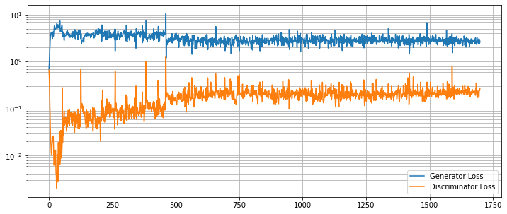
MONAI 0.7 : tutorials : モジュール – MedNIST で GAN
このノートブックはランダムな入力テンソルから画像を生成するネットワークを訓練するための MONAI の使用方法を示します。単純な GAN は別々の Generator と Discriminator ネットワークで済ませます。
これは以下のステップを通り抜けます :
- 遠隔ソースからデータをロードする
- このデータからのデータセットと変換を構築する
- ネットワークを定義する
- 訓練と評価
環境セットアップ
!python -c "import monai" || pip install -q monai-weekly
!python -c "import matplotlib" || pip install -q matplotlib
%matplotlib inline
from monai.utils import progress_bar, set_determinism
from monai.transforms import (
    AddChannel,
    Compose,
    RandFlip,
    RandRotate,
    RandZoom,
    ScaleIntensity,
    EnsureType,
    Transform,
)
from monai.networks.nets import Discriminator, Generator
from monai.networks import normal_init
from monai.data import CacheDataset
from monai.config import print_config
from monai.apps import download_and_extract
import numpy as np
import torch
import matplotlib.pyplot as plt
import os
import tempfile
インポートのセットアップ
# Copyright 2020 MONAI Consortium
# Licensed under the Apache License, Version 2.0 (the "License");
# you may not use this file except in compliance with the License.
# You may obtain a copy of the License at
#     http://www.apache.org/licenses/LICENSE-2.0
# Unless required by applicable law or agreed to in writing, software
# distributed under the License is distributed on an "AS IS" BASIS,
# WITHOUT WARRANTIES OR CONDITIONS OF ANY KIND, either express or implied.
# See the License for the specific language governing permissions and
# limitations under the License.


print_config()
MONAI version: 0.6.0rc1+23.gc6793fd0
Numpy version: 1.20.3
Pytorch version: 1.9.0a0+c3d40fd
MONAI flags: HAS_EXT = True, USE_COMPILED = False
MONAI rev id: c6793fd0f316a448778d0047664aaf8c1895fe1c

Optional dependencies:
Pytorch Ignite version: 0.4.5
Nibabel version: 3.2.1
scikit-image version: 0.15.0
Pillow version: 7.0.0
Tensorboard version: 2.5.0
gdown version: 3.13.0
TorchVision version: 0.10.0a0
ITK version: 5.1.2
tqdm version: 4.53.0
lmdb version: 1.2.1
psutil version: 5.8.0
pandas version: 1.1.4
einops version: 0.3.0

For details about installing the optional dependencies, please visit:
    https://docs.monai.io/en/latest/installation.html#installing-the-recommended-dependencies
再現性のための決定論的訓練
set_determinism(seed=0)
訓練変数の定義
disc_train_interval = 1
disc_train_steps = 5
batch_size = 300
latent_size = 64
max_epochs = 50
real_label = 1
gen_label = 0
learning_rate = 2e-4
betas = (0.5, 0.999)
データディレクトリのセットアップ
MONAI_DATA_DIRECTORY 環境変数でディレクトリを指定できます。これは結果をセーブしてダウンロードを再利用することを可能にします。指定されない場合、一時ディレクトリが使用されます。
directory = os.environ.get("MONAI_DATA_DIRECTORY")
root_dir = tempfile.mkdtemp() if directory is None else directory
print(root_dir)
/workspace/data/medical
データセットをダウンロードする
MedMNIST データセットは TCIA, RSNA Bone Age チャレンジ と NIH Chest X-ray データセット からの様々なセットから集められました。
データセットは Dr. Bradley J. Erickson M.D., Ph.D. (Department of Radiology, Mayo Clinic) のお陰により Creative Commons CC BY-SA 4.0 ライセンス のもとで利用可能になっています。
MedNIST データセットを使用する場合、出典を明示してください、e.g. https://github.com/Project-MONAI/tutorials/blob/master/2d_classification/mednist_tutorial.ipynb。
ここではファイルシステムを使用することなく tar ファイルからダウンロードして読む方法を示すためと、ハンド X-rays の画像だけを望むために、遠隔ソースからデータをロードする方法は異なります。これは分類サンプルではないのでカテゴリーデータは必要ありませんので、tarball をダウンロードし、標準ライブラリを使用してそれをオープンし、そしてハンドのためのファイル名の総てを recall します :
resource = "https://drive.google.com/uc?id=1QsnnkvZyJPcbRoV_ArW8SnE1OTuoVbKE"
md5 = "0bc7306e7427e00ad1c5526a6677552d"

compressed_file = os.path.join(root_dir, "MedNIST.tar.gz")
data_dir = os.path.join(root_dir, "MedNIST")
if not os.path.exists(data_dir):
    download_and_extract(resource, compressed_file, root_dir, md5)

hands = [
    os.path.join(data_dir, "Hand", x)
    for x in os.listdir(os.path.join(data_dir, "Hand"))
]
tarfile から実際の画像データをロードするため、Matplotlib を使用してこれを行なう変換タイプを定義します。これはデータを準備するために他の変換とともに使用され、ランダム化された増強変換が続きます。ここでは tarball からの準備された画像の総てをキャッシュするために CacheDataset クラスが使用されますので、ランダム化された回転、反転とズーム操作により増強される予定の準備された画像の総てをメモリ持ちます :
class LoadTarJpeg(Transform):
    def __call__(self, data):
        return plt.imread(data)


train_transforms = Compose(
    [
        LoadTarJpeg(),
        AddChannel(),
        ScaleIntensity(),
        RandRotate(range_x=np.pi / 12, prob=0.5, keep_size=True),
        RandFlip(spatial_axis=0, prob=0.5),
        RandZoom(min_zoom=0.9, max_zoom=1.1, prob=0.5),
        EnsureType(),
    ]
)

train_ds = CacheDataset(hands, train_transforms)
train_loader = torch.utils.data.DataLoader(
    train_ds, batch_size=batch_size, shuffle=True, num_workers=10
)
100%|██████████| 10000/10000 [00:05<00:00, 1691.00it/s]
今は generator と discriminator ネットワークを定義します。パラメータは tar ファイルからロードされた (1, 64, 64) の画像サイズに合うように注意深く選択されています。discriminator への入力画像は非常に小さい画像を生成するために 4 回ダウンサンプリングされます、これらは平坦化されて完全結合層への入力として渡されます。generator への入力潜在ベクトルは shape (64, 8, 8) の出力を生成するために完全結合層に渡されます、そしてこれはリアル画像と同じ shape である最終的な出力を生成するために 3 回アップサンプリングされます。結果を改善するためにネットワークは正規化スキームで初期化されます :
device = torch.device("cuda:0")
disc_net = Discriminator(
    in_shape=(1, 64, 64),
    channels=(8, 16, 32, 64, 1),
    strides=(2, 2, 2, 2, 1),
    num_res_units=1,
    kernel_size=5,
).to(device)


gen_net = Generator(
    latent_shape=latent_size, start_shape=(64, 8, 8),
    channels=[32, 16, 8, 1], strides=[2, 2, 2, 1],
)

# initialize both networks
disc_net.apply(normal_init)
gen_net.apply(normal_init)

# input images are scaled to [0,1] so enforce the same of generated outputs
gen_net.conv.add_module("activation", torch.nn.Sigmoid())
gen_net = gen_net.to(device)
今は generator と discriminator のための損失計算プロレスをラップするヘルパー関数とともに使用する損失関数を定義します。optimizer もまた定義します :
disc_loss = torch.nn.BCELoss()
gen_loss = torch.nn.BCELoss()

disc_opt = torch.optim.Adam(disc_net.parameters(), learning_rate, betas=betas)
gen_opt = torch.optim.Adam(gen_net.parameters(), learning_rate, betas=betas)


def discriminator_loss(gen_images, real_images):
    """
    The discriminator loss if calculated by comparing its
    prediction for real and generated images.

    """
    real = real_images.new_full((real_images.shape[0], 1), real_label)
    gen = gen_images.new_full((gen_images.shape[0], 1), gen_label)

    realloss = disc_loss(disc_net(real_images), real)
    genloss = disc_loss(disc_net(gen_images.detach()), gen)

    return (realloss + genloss) / 2


def generator_loss(input):
    """
    The generator loss is calculated by determining how well
    the discriminator was fooled by the generated images.

    """
    output = disc_net(input)
    cats = output.new_full(output.shape, real_label)
    return gen_loss(output, cats)
今は幾つかのエポックの間データセットに渡り反復することにより訓練します。各バッチのための generator 訓練ステージの後、discriminator は同じリアルと生成画像上で幾つかのステップの間訓練されます。
epoch_loss_values = [(0, 0)]
gen_step_loss = []
disc_step_loss = []
step = 0

for epoch in range(max_epochs):
    gen_net.train()
    disc_net.train()
    epoch_loss = 0

    for i, batch_data in enumerate(train_loader):
        progress_bar(
            i, len(
                train_loader),
            f"epoch {epoch + 1}, avg loss: {epoch_loss_values[-1][1]:.4f}",
        )
        real_images = batch_data.to(device)
        latent = torch.randn(real_images.shape[0], latent_size).to(device)

        gen_opt.zero_grad()
        gen_images = gen_net(latent)
        loss = generator_loss(gen_images)
        loss.backward()
        gen_opt.step()
        epoch_loss += loss.item()

        gen_step_loss.append((step, loss.item()))

        if step % disc_train_interval == 0:
            disc_total_loss = 0

            for _ in range(disc_train_steps):
                disc_opt.zero_grad()
                dloss = discriminator_loss(gen_images, real_images)
                dloss.backward()
                disc_opt.step()
                disc_total_loss += dloss.item()

            disc_step_loss.append((step, disc_total_loss / disc_train_steps))

        step += 1

    epoch_loss /= step
    epoch_loss_values.append((step, epoch_loss))
33/34 epoch 50, avg loss: 0.0563 [============================= ]
generator と discriminator のための個別の損失値は一緒にグラフ化できます。これらは、discriminator を騙す generator の能力がリアルとフェイク画像の間を正確に識別するネットワークの能力と均衡するにつれて、均衡に達するはずです。
plt.figure(figsize=(12, 5))
plt.semilogy(*zip(*gen_step_loss), label="Generator Loss")
plt.semilogy(*zip(*disc_step_loss), label="Discriminator Loss")
plt.grid(True, "both", "both")
plt.legend()
最後に幾つかランダムに生成された画像を示します。望ましくは期待されるように殆どの画像が 4 本の指と親指を持つことです (polydactyl (= 多指の) サンプルがデータセットに多くは存在していないと仮定して)。このデモ目的のノートブックは長くはネットワークを訓練しません、デフォルトの 50 エポックを越えた訓練は結果を改善するはずです。
test_size = 10
test_latent = torch.randn(test_size, latent_size).to(device)

test_images = gen_net(test_latent)

fig, axs = plt.subplots(1, test_size, figsize=(20, 4))

for i, ax in enumerate(axs):
    ax.axis("off")
    ax.imshow(test_images[i, 0].cpu().data.numpy(), cmap="gray")

以上
MONAI 0.7 : tutorials : 2D レジストレーション – 2D XRay レジストレーション・デモ
MONAI 0.7 : tutorials : 2D レジストレーション – 2D XRay レジストレーション・デモ (翻訳/解説)
翻訳 : (株)クラスキャット セールスインフォメーション
作成日時 : 10/10/2021 (0.7.0)
* 本ページは、MONAI の以下のドキュメントを翻訳した上で適宜、補足説明したものです:
* サンプルコードの動作確認はしておりますが、必要な場合には適宜、追加改変しています。
* ご自由にリンクを張って頂いてかまいませんが、sales-info@classcat.com までご一報いただけると嬉しいです。
- 人工知能研究開発支援
- 人工知能研修サービス(経営者層向けオンサイト研修)
- テクニカルコンサルティングサービス
- 実証実験(プロトタイプ構築)
- アプリケーションへの実装
- 人工知能研修サービス
- PoC(概念実証)を失敗させないための支援
- テレワーク & オンライン授業を支援
- お住まいの地域に関係なく Web ブラウザからご参加頂けます。事前登録 が必要ですのでご注意ください。
- ウェビナー運用には弊社製品「ClassCat® Webinar」を利用しています。
◆ お問合せ : 本件に関するお問い合わせ先は下記までお願いいたします。
| 株式会社クラスキャット セールス・マーケティング本部 セールス・インフォメーション |
| E-Mail:sales-info@classcat.com ; WebSite: https://www.classcat.com/ ; Facebook |
MONAI 0.7 : tutorials : 2D レジストレーション – 2D XRay レジストレーション・デモ
このノートブックは学習ベースの 64 x 64 X-Ray ハンドのアフィン・レジストレーションの素早いデモを示します。
このデモは MONAI のレジストレーション機能の使用方法を示す toy サンプルです。
このデモは主として以下を使用します :
- アフィン変換パラメータを予測するためにアフィンヘッドを持つ UNet ライクなレジストレーション・ネットワーク ;
- moving 画像を変換するための、MONAI C++/CUDA として実装された、warp 関数。
環境のセットアップ
BUILD_MONAI=1 フラグで “pip install” すると、MONA レポジトリから最新のソースコードを取得し、MONAI の C++/CUDA 拡張を構築して、パッケージをインストールします。
env BUILD_MONAI=1 の設定は、関連する Python モジュールを呼び出すとき MONAI は Pytorch/Python ネイティブ実装の代わりにそれらの拡張を優先することを示します。
(コンパイルは数分から 10+ 分かかる場合があります。)
%env BUILD_MONAI=1
!python -c "import monai" || pip install -q git+https://github.com/Project-MONAI/MONAI#egg=monai[all]
インポートのセットアップ
from monai.utils import set_determinism, first
from monai.transforms import (
    EnsureChannelFirstD,
    Compose,
    LoadImageD,
    RandRotateD,
    RandZoomD,
    ScaleIntensityRanged,
    EnsureTypeD,
)
from monai.data import DataLoader, Dataset, CacheDataset
from monai.config import print_config, USE_COMPILED
from monai.networks.nets import GlobalNet
from monai.networks.blocks import Warp
from monai.apps import MedNISTDataset

import numpy as np
import torch
from torch.nn import MSELoss
import matplotlib.pyplot as plt


print_config()
set_determinism(42)
MONAI version: 0.5.0+7.g9f4da6a
Numpy version: 1.19.5
Pytorch version: 1.8.1+cu101
MONAI flags: HAS_EXT = True, USE_COMPILED = True
MONAI rev id: 9f4da6acded249bba24c85eaee4ece256ed45815

Optional dependencies:
Pytorch Ignite version: 0.4.4
Nibabel version: 3.0.2
scikit-image version: 0.16.2
Pillow version: 7.1.2
Tensorboard version: 2.4.1
gdown version: 3.6.4
TorchVision version: 0.9.1+cu101
ITK version: 5.1.2
tqdm version: 4.60.0
lmdb version: 0.99
psutil version: 5.4.8

For details about installing the optional dependencies, please visit:
    https://docs.monai.io/en/latest/installation.html#installing-the-recommended-dependencies
ペア単位の訓練入力の構築
実際のデータファイルをダウンロードして unzip するために MedNISTDataset オブジェクトを使用します。そして hand クラスを選択し、ロードされたデータ辞書を “fixed_hand” と “moving_hand” に変換します、これらは合成訓練ペアを作成するために別々に前処理されます。
train_data = MedNISTDataset(root_dir="./", section="training", download=True, transform=None)
training_datadict = [
    {"fixed_hand": item["image"], "moving_hand": item["image"]}
    for item in train_data.data if item["label"] == 4  # label 4 is for xray hands
]
print("\n first training items: ", training_datadict[:3])
MedNIST.tar.gz: 59.0MB [00:07, 8.83MB/s]
downloaded file: ./MedNIST.tar.gz.
Verified 'MedNIST.tar.gz', md5: 0bc7306e7427e00ad1c5526a6677552d.
Verified 'MedNIST.tar.gz', md5: 0bc7306e7427e00ad1c5526a6677552d.
Loading dataset: 100%|██████████| 47164/47164 [00:00<00:00, 145309.19it/s]
 first training items:  [{'fixed_hand': './MedNIST/Hand/003696.jpeg', 'moving_hand': './MedNIST/Hand/003696.jpeg'}, {'fixed_hand': './MedNIST/Hand/001404.jpeg', 'moving_hand': './MedNIST/Hand/001404.jpeg'}, {'fixed_hand': './MedNIST/Hand/008882.jpeg', 'moving_hand': './MedNIST/Hand/008882.jpeg'}]
train_transforms = Compose(
    [
        LoadImageD(keys=["fixed_hand", "moving_hand"]),
        EnsureChannelFirstD(keys=["fixed_hand", "moving_hand"]),
        ScaleIntensityRanged(keys=["fixed_hand", "moving_hand"],
                             a_min=0., a_max=255., b_min=0.0, b_max=1.0, clip=True,),
        RandRotateD(keys=["moving_hand"], range_x=np.pi/4, prob=1.0, keep_size=True, mode="bicubic"),
        RandZoomD(keys=["moving_hand"], min_zoom=0.9, max_zoom=1.1, prob=1.0, mode="bicubic", align_corners=False),
        EnsureTypeD(keys=["fixed_hand", "moving_hand"]),
    ]
)
訓練ペアの可視化
check_ds = Dataset(data=training_datadict, transform=train_transforms)
check_loader = DataLoader(check_ds, batch_size=1, shuffle=True)
check_data = first(check_loader)
fixed_image = check_data["fixed_hand"][0][0]
moving_image = check_data["moving_hand"][0][0]

print(f"moving_image shape: {moving_image.shape}")
print(f"fixed_image shape: {fixed_image.shape}")

plt.figure("check", (12, 6))
plt.subplot(1, 2, 1)
plt.title("moving_image")
plt.imshow(moving_image, cmap="gray")
plt.subplot(1, 2, 2)
plt.title("fixed_image")
plt.imshow(fixed_image, cmap="gray")

plt.show()
moving_image shape: torch.Size([64, 64])
fixed_image shape: torch.Size([64, 64])
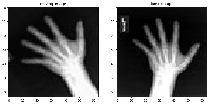
訓練パイプラインを作成する
訓練ペアを獲得して訓練プロセスを高速化するために CacheDataset を使用します。この訓練データは GlobalNet に供給されます、これは 画像レベルのアフィン変換パラメータを予測します。Warp 層は初期化されて訓練と推論の両方のために使用されます。
train_ds = CacheDataset(data=training_datadict[:1000], transform=train_transforms,
                        cache_rate=1.0, num_workers=4)
train_loader = DataLoader(train_ds, batch_size=16, shuffle=True, num_workers=2)
Loading dataset: 100%|██████████| 1000/1000 [00:01<00:00, 558.34it/s]
device = torch.device("cuda:0")
model = GlobalNet(
    image_size=(64, 64),
    spatial_dims=2,
    in_channels=2,  # moving and fixed
    num_channel_initial=16,
    depth=3).to(device)
image_loss = MSELoss()
if USE_COMPILED:
    warp_layer = Warp(3, "border").to(device)
else:
    warp_layer = Warp("bilinear", "border").to(device)
optimizer = torch.optim.Adam(model.parameters(), 1e-5)
訓練ループ
max_epochs = 200
epoch_loss_values = []

for epoch in range(max_epochs):
    print("-" * 10)
    print(f"epoch {epoch + 1}/{max_epochs}")
    model.train()
    epoch_loss, step = 0, 0
    for batch_data in train_loader:
        step += 1
        optimizer.zero_grad()

        moving = batch_data["moving_hand"].to(device)
        fixed = batch_data["fixed_hand"].to(device)
        ddf = model(torch.cat((moving, fixed), dim=1))
        pred_image = warp_layer(moving, ddf)

        loss = image_loss(pred_image, fixed)
        loss.backward()
        optimizer.step()
        epoch_loss += loss.item()
        # print(f"{step}/{len(train_ds) // train_loader.batch_size}, "
        #       f"train_loss: {loss.item():.4f}")

    epoch_loss /= step
    epoch_loss_values.append(epoch_loss)
    print(f"epoch {epoch + 1} average loss: {epoch_loss:.4f}")
%matplotlib inline
plt.plot(epoch_loss_values)
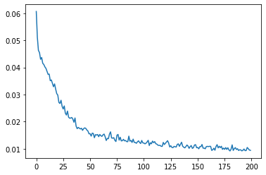
幾つかの検証結果の視覚化
このセクションは moving vs fixed ハンドの初見の (i.e. 前に見てない) ペアのセットを作成して各ペアの間の変換を予測するためにネットワークを使用します。
val_ds = CacheDataset(data=training_datadict[2000:2500], transform=train_transforms,
                      cache_rate=1.0, num_workers=0)
val_loader = DataLoader(val_ds, batch_size=16, num_workers=0)
for batch_data in val_loader:
    moving = batch_data["moving_hand"].to(device)
    fixed = batch_data["fixed_hand"].to(device)
    ddf = model(torch.cat((moving, fixed), dim=1))
    pred_image = warp_layer(moving, ddf)
    break

fixed_image = fixed.detach().cpu().numpy()[:, 0]
moving_image = moving.detach().cpu().numpy()[:, 0]
pred_image = pred_image.detach().cpu().numpy()[:, 0]
Loading dataset: 100%|██████████| 500/500 [00:00<00:00, 803.96it/s]
%matplotlib inline
batch_size = 5
plt.subplots(batch_size, 3, figsize=(8, 10))
for b in range(batch_size):
    # moving image
    plt.subplot(batch_size, 3, b * 3 + 1)
    plt.axis('off')
    plt.title("moving image")
    plt.imshow(moving_image[b], cmap="gray")
    # fixed image
    plt.subplot(batch_size, 3, b * 3 + 2)
    plt.axis('off')
    plt.title("fixed image")
    plt.imshow(fixed_image[b], cmap="gray")
    # warped moving
    plt.subplot(batch_size, 3, b * 3 + 3)
    plt.axis('off')
    plt.title("predicted image")
    plt.imshow(pred_image[b], cmap="gray")
plt.axis('off')
plt.show()
以上
MONAI 0.7 : tutorials : モジュール – MedNIST データセットによる Autoencoder ネットワーク
MONAI 0.7 : tutorials : モジュール – MedNIST データセットによる Autoencoder ネットワーク (翻訳/解説)
翻訳 : (株)クラスキャット セールスインフォメーション
作成日時 : 10/09/2021 (0.7.0)
* 本ページは、MONAI の以下のドキュメントを翻訳した上で適宜、補足説明したものです:
* サンプルコードの動作確認はしておりますが、必要な場合には適宜、追加改変しています。
* ご自由にリンクを張って頂いてかまいませんが、sales-info@classcat.com までご一報いただけると嬉しいです。
- 人工知能研究開発支援
- 人工知能研修サービス(経営者層向けオンサイト研修)
- テクニカルコンサルティングサービス
- 実証実験(プロトタイプ構築)
- アプリケーションへの実装
- 人工知能研修サービス
- PoC(概念実証)を失敗させないための支援
- テレワーク & オンライン授業を支援
- お住まいの地域に関係なく Web ブラウザからご参加頂けます。事前登録 が必要ですのでご注意ください。
- ウェビナー運用には弊社製品「ClassCat® Webinar」を利用しています。
◆ お問合せ : 本件に関するお問い合わせ先は下記までお願いいたします。
| 株式会社クラスキャット セールス・マーケティング本部 セールス・インフォメーション |
| E-Mail:sales-info@classcat.com ; WebSite: https://www.classcat.com/ ; Facebook |
MONAI 0.7 : tutorials : モジュール – MedNIST データセットによる Autoencoder ネットワーク
このチュートリアルは MONAI の autoencoder クラスを実演するために MedNIST ハンド CT スキャン・データセットを使用します。autoencoder は恒等エンコード/デコードで使用され (i.e. 入れたものが戻されるべきもの)、そしてぼかしやノイズの除去の使用方法として実演します。
このノートブックは画像のぼかし/ノイズ除去の目的で MONAI で autoencoeder の使用を示します。
学習目標
これは以下のステップを通り抜けます :
- 遠隔ソースからデータをロードする
- 画像の辞書を作成するために lambda を使用する
- MONAI の組込み AutoEncoder を使用する
環境のセットアップ
!python -c "import monai" || pip install -q "monai-weekly[pillow, tqdm]"
1. インポートと設定
import logging
import os
import shutil
import sys
import tempfile
import random
import numpy as np
from tqdm import trange
import matplotlib.pyplot as plt
import torch
from skimage.util import random_noise

from monai.apps import download_and_extract
from monai.config import print_config
from monai.data import CacheDataset, DataLoader
from monai.networks.nets import AutoEncoder
from monai.transforms import (
    AddChannelD,
    Compose,
    LoadImageD,
    RandFlipD,
    RandRotateD,
    RandZoomD,
    ScaleIntensityD,
    EnsureTypeD,
    Lambda,
)
from monai.utils import set_determinism

print_config()
MONAI version: 0.6.0rc1+23.gc6793fd0
Numpy version: 1.20.3
Pytorch version: 1.9.0a0+c3d40fd
MONAI flags: HAS_EXT = True, USE_COMPILED = False
MONAI rev id: c6793fd0f316a448778d0047664aaf8c1895fe1c

Optional dependencies:
Pytorch Ignite version: 0.4.5
Nibabel version: 3.2.1
scikit-image version: 0.15.0
Pillow version: 8.2.0
Tensorboard version: 2.5.0
gdown version: 3.13.0
TorchVision version: 0.10.0a0
ITK version: 5.1.2
tqdm version: 4.53.0
lmdb version: 1.2.1
psutil version: 5.8.0
pandas version: 1.1.4
einops version: 0.3.0

For details about installing the optional dependencies, please visit:
    https://docs.monai.io/en/latest/installation.html#installing-the-recommended-dependencies
logging.basicConfig(stream=sys.stdout, level=logging.INFO)
set_determinism(0)
device = torch.device("cuda" if torch.cuda.is_available() else "cpu")
# Create small visualistaion function
def plot_ims(ims, shape=None, figsize=(10, 10), titles=None):
    shape = (1, len(ims)) if shape is None else shape
    plt.subplots(*shape, figsize=figsize)
    for i, im in enumerate(ims):
        plt.subplot(*shape, i + 1)
        im = plt.imread(im) if isinstance(im, str) else torch.squeeze(im)
        plt.imshow(im, cmap='gray')
        if titles is not None:
            plt.title(titles[i])
        plt.axis('off')
    plt.tight_layout()
    plt.show()
データを取得する
MedMNIST データセットは TCIA, RSNA Bone Age チャレンジ と NIH Chest X-ray データセット からの様々なセットから集められました。
データセットは Dr. Bradley J. Erickson M.D., Ph.D. (Department of Radiology, Mayo Clinic) のお陰により Creative Commons CC BY-SA 4.0 ライセンス のもとで利用可能になっています。
directory = os.environ.get("MONAI_DATA_DIRECTORY")
root_dir = tempfile.mkdtemp() if directory is None else directory
print(root_dir)
/workspace/data/medical
resource = "https://drive.google.com/uc?id=1QsnnkvZyJPcbRoV_ArW8SnE1OTuoVbKE"
md5 = "0bc7306e7427e00ad1c5526a6677552d"

compressed_file = os.path.join(root_dir, "MedNIST.tar.gz")
data_dir = os.path.join(root_dir, "MedNIST")
if not os.path.exists(data_dir):
    download_and_extract(resource, compressed_file, root_dir, md5)
# scan_type could be  AbdomenCT  BreastMRI  CXR  ChestCT  Hand  HeadCT
scan_type = "Hand"
im_dir = os.path.join(data_dir, scan_type)
all_filenames = [os.path.join(im_dir, filename)
                 for filename in os.listdir(im_dir)]
random.shuffle(all_filenames)

# Visualise a few of them
rand_images = np.random.choice(all_filenames, 8, replace=False)
plot_ims(rand_images, shape=(2, 4))
# Split into training and testing
test_frac = 0.2
num_test = int(len(all_filenames) * test_frac)
num_train = len(all_filenames) - num_test
train_datadict = [{"im": fname} for fname in all_filenames[:num_train]]
test_datadict = [{"im": fname} for fname in all_filenames[-num_test:]]
print(f"total number of images: {len(all_filenames)}")
print(f"number of images for training: {len(train_datadict)}")
print(f"number of images for testing: {len(test_datadict)}")
total number of images: 10000
number of images for training: 8000
number of images for testing: 2000
3. 画像変換チェインを作成する
画像のぼやけ/ノイズを除去するために autoencoder を訓練するため、劣化画像をエンコーダに渡すことを望みますが、損失関数では、元の、劣化していないバージョンとの比較を行ないます。この意味で、エンコードとデコードステップが劣化を除去できたときに、損失関数は最小化されます。
画像の一つのバージョンが劣化していて他方がそうではないという事実以外に、それらが同一であるようにすることを望みます、これは同じ変換から生成される必要があることを意味します。これを行なう最も簡単な方法は辞書変換を介することです、そこでは最後に、3 つの画像- オリジナル、ガウスぼかしとノイズのある (画像) を含む辞書を返す lambda 関数をもちます。
NoiseLambda = Lambda(lambda d: {
    "orig": d["im"],
    "gaus": torch.tensor(
        random_noise(d["im"], mode='gaussian'), dtype=torch.float32),
    "s&p": torch.tensor(random_noise(d["im"], mode='s&p', salt_vs_pepper=0.1)),
})

train_transforms = Compose(
    [
        LoadImageD(keys=["im"]),
        AddChannelD(keys=["im"]),
        ScaleIntensityD(keys=["im"]),
        RandRotateD(keys=["im"], range_x=np.pi / 12, prob=0.5, keep_size=True),
        RandFlipD(keys=["im"], spatial_axis=0, prob=0.5),
        RandZoomD(keys=["im"], min_zoom=0.9, max_zoom=1.1, prob=0.5),
        EnsureTypeD(keys=["im"]),
        NoiseLambda,
    ]
)

test_transforms = Compose(
    [
        LoadImageD(keys=["im"]),
        AddChannelD(keys=["im"]),
        ScaleIntensityD(keys=["im"]),
        EnsureTypeD(keys=["im"]),
        NoiseLambda,
    ]
)
データセットとデーたローダを作成する
データを保持して訓練の間にバッチを提示する
batch_size = 300
num_workers = 10

train_ds = CacheDataset(train_datadict, train_transforms,
                        num_workers=num_workers)
train_loader = DataLoader(train_ds, batch_size=batch_size,
                          shuffle=True, num_workers=num_workers)
test_ds = CacheDataset(test_datadict, test_transforms, num_workers=num_workers)
test_loader = DataLoader(test_ds, batch_size=batch_size,
                         shuffle=True, num_workers=num_workers)
100%|██████████| 8000/8000 [00:02<00:00, 2698.01it/s]
100%|██████████| 2000/2000 [00:02<00:00, 904.36it/s]
# Get image original and its degraded versions
def get_single_im(ds):
    loader = torch.utils.data.DataLoader(
        ds, batch_size=1, num_workers=10, shuffle=True)
    itera = iter(loader)
    return next(itera)
data = get_single_im(train_ds)
plot_ims([data['orig'], data['gaus'], data['s&p']],
         titles=['orig', 'Gaussian', 's&p'])
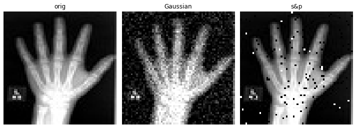
def train(dict_key_for_training, max_epochs=10, learning_rate=1e-3):

    model = AutoEncoder(
        spatial_dims=2,
        in_channels=1,
        out_channels=1,
        channels=(4, 8, 16, 32),
        strides=(2, 2, 2, 2),
    ).to(device)

    # Create loss fn and optimiser
    loss_function = torch.nn.MSELoss()
    optimizer = torch.optim.Adam(model.parameters(), learning_rate)

    epoch_loss_values = []

    t = trange(
        max_epochs,
        desc=f"{dict_key_for_training} -- epoch 0, avg loss: inf", leave=True)
    for epoch in t:
        model.train()
        epoch_loss = 0
        step = 0
        for batch_data in train_loader:
            step += 1
            inputs = batch_data[dict_key_for_training].to(device)
            optimizer.zero_grad()
            outputs = model(inputs)
            loss = loss_function(outputs, batch_data['orig'].to(device))
            loss.backward()
            optimizer.step()
            epoch_loss += loss.item()
        epoch_loss /= step
        epoch_loss_values.append(epoch_loss)
        t.set_description(
            f"{dict_key_for_training} -- epoch {epoch + 1}"
            + f", average loss: {epoch_loss:.4f}")
    return model, epoch_loss_values
max_epochs = 50
training_types = ['orig', 'gaus', 's&p']
models = []
epoch_losses = []
for training_type in training_types:
    model, epoch_loss = train(training_type, max_epochs=max_epochs)
    models.append(model)
    epoch_losses.append(epoch_loss)
orig -- epoch 30, average loss: 0.0110: 60%|██████ | 30/50 [01:41<01:08, 3.40s/it]
plt.figure()
plt.title("Epoch Average Loss")
plt.xlabel("epoch")
for y, label in zip(epoch_losses, training_types):
    x = list(range(1, len(y) + 1))
    line, = plt.plot(x, y)
    line.set_label(label)
plt.legend()
data = get_single_im(test_ds)

recons = []
for model, training_type in zip(models, training_types):
    im = data[training_type]
    recon = model(im.to(device)).detach().cpu()
    recons.append(recon)

plot_ims(
    [data['orig'], data['gaus'], data['s&p']] + recons,
    titles=['orig', 'Gaussian', 'S&P'] +
    ["recon w/\n" + x for x in training_types],
    shape=(2, len(training_types)))
データディレクトリのクリーンアップ
一時ディレクトリが使用された場合ディレクトリを削除します。
if directory is None:
    shutil.rmtree(root_dir)
以上
ClassCat® Chatbot
人工知能開発支援
- テクニカルコンサルティングサービス
- 実証実験 (プロトタイプ構築)
- アプリケーションへの実装
- 人工知能研修サービス
クラスキャット
セールス・インフォメーション
E-Mail:sales-info@classcat.com