ホーム » sales-info の投稿 (ページ 3)

作者アーカイブ: sales-info

MONAI 0.7 : tutorials : 3D セグメンテーション – MONAI と Catalyst による 3D セグメンテーション

10/22/2021

MONAI 0.7 : tutorials : 3D セグメンテーション – MONAI と Catalyst による 3D セグメンテーション (翻訳/解説)

翻訳 : (株)クラスキャットセールスインフォメーション
作成日時 : 10/22/2021 (0.7.0)

* 本ページは、MONAI の以下のドキュメントを翻訳した上で適宜、補足説明したものです：

3D segmentation with MONAI and Catalyst

* サンプルコードの動作確認はしておりますが、必要な場合には適宜、追加改変しています。
* ご自由にリンクを張って頂いてかまいませんが、sales-info@classcat.com までご一報いただけると嬉しいです。

クラスキャット人工知能研究開発支援サービス ★ 無料 Web セミナー開催中 ★

◆ クラスキャットは人工知能・テレワークに関する各種サービスを提供しております。お気軽にご相談ください :

人工知能研究開発支援
1. 人工知能研修サービス(経営者層向けオンサイト研修)
2. テクニカルコンサルティングサービス
3. 実証実験(プロトタイプ構築)
4. アプリケーションへの実装
人工知能研修サービス
PoC(概念実証)を失敗させないための支援
テレワーク & オンライン授業を支援

◆ 人工知能とビジネスをテーマに WEB セミナーを定期的に開催しています。スケジュール。

お住まいの地域に関係なく Web ブラウザからご参加頂けます。事前登録 が必要ですのでご注意ください。
ウェビナー運用には弊社製品「ClassCat® Webinar」を利用しています。

◆ お問合せ : 本件に関するお問い合わせ先は下記までお願いいたします。

株式会社クラスキャット セールス・マーケティング本部セールス・インフォメーション

E-Mail：sales-info@classcat.com ; WebSite: https://www.classcat.com/ ; Facebook

MONAI 0.7 : tutorials : 3D セグメンテーション – MONAI と Catalyst による 3D セグメンテーション

このノートブックは MONAI が Catalyst フレームワークと連携して使用される場合の方法を示します。

このチュートリアルは、3D セグメンテーション・タスクのために MONAI を Catalyst フレームワークと共に使用できる方法を実演します。そして以下の機能を簡単に利用できます :

合成データを準備する。
メタデータと一緒に Nifti 画像をロードする。
辞書形式データのための変換。
チャネル次元がない場合、データにチャネル dim を追加する。
医療画像強度を想定される範囲でスケールする。
ポジティブ / ネガティブ・ラベル比率に基づいてバランスの取れた画像のバッチをクロップする。
3D セグメンテーション・タスクのための 3D UNet モデル、Dice 損失関数、Mean Dice メトリック。
スライディング・ウィンドウ推論法。
再現性のための決定論的訓練。

このチュートリアルは unet_training_dict.py と spleen_segmentation_3d.ipynb に基づいています。

環境のセットアップ

!python -c "import monai" || pip install -q "monai-weekly[nibabel, tensorboard]"
!python -c "import matplotlib" || pip install -q matplotlib
!python -c "import catalyst" || pip install -q catalyst==20.07
%matplotlib inline

インポートのセットアップ

# Copyright 2020 MONAI Consortium
# Licensed under the Apache License, Version 2.0 (the "License");
# you may not use this file except in compliance with the License.
# You may obtain a copy of the License at
#     http://www.apache.org/licenses/LICENSE-2.0
# Unless required by applicable law or agreed to in writing, software
# distributed under the License is distributed on an "AS IS" BASIS,
# WITHOUT WARRANTIES OR CONDITIONS OF ANY KIND, either express or implied.
# See the License for the specific language governing permissions and
# limitations under the License.

import glob
import logging
import os
import shutil
import sys
import tempfile

import catalyst.dl
import matplotlib.pyplot as plt
import nibabel as nib
import numpy as np
from monai.config import print_config
from monai.data import Dataset, create_test_image_3d, list_data_collate, decollate_batch
from monai.inferers import sliding_window_inference
from monai.losses import DiceLoss
from monai.metrics import DiceMetric
from monai.networks.nets import UNet
from monai.transforms import (
    Activations,
    AsChannelFirstd,
    AsDiscrete,
    Compose,
    LoadImaged,
    RandCropByPosNegLabeld,
    RandRotate90d,
    ScaleIntensityd,
    EnsureTyped,
    EnsureType,
)
from monai.utils import first

import torch

print_config()

MONAI version: 0.6.0rc1+2.g50d83912
Numpy version: 1.20.1
Pytorch version: 1.9.0a0+2ecb2c7
MONAI flags: HAS_EXT = True, USE_COMPILED = False
MONAI rev id: 50d83912536c5579506cdf6920c47ba65ea66e49

Optional dependencies:
Pytorch Ignite version: 0.4.5
Nibabel version: 3.2.1
scikit-image version: 0.15.0
Pillow version: 8.2.0
Tensorboard version: 1.15.0+nv
gdown version: 3.13.0
TorchVision version: 0.9.0a0
ITK version: 5.1.2
tqdm version: 4.53.0
lmdb version: 1.2.1
psutil version: 5.8.0
pandas version: 1.1.4

For details about installing the optional dependencies, please visit:
    https://docs.monai.io/en/latest/installation.html#installing-the-recommended-dependencies

データディレクトリのセットアップ

MONAI_DATA_DIRECTORY 環境変数でディレクトリを指定できます。これは結果をセーブしてダウンロードを再利用することを可能にします。指定されない場合、一時ディレクトリが使用されます。

directory = os.environ.get("MONAI_DATA_DIRECTORY")
root_dir = tempfile.mkdtemp() if directory is None else directory
print(root_dir)

/workspace/data/medical

ロギングのセットアップ

logging.basicConfig(stream=sys.stdout, level=logging.INFO)

MONAI コンポーネント

合成データの準備

for i in range(40):
    im, seg = create_test_image_3d(
        128, 128, 128, num_seg_classes=1, channel_dim=-1
    )

    n = nib.Nifti1Image(im, np.eye(4))
    nib.save(n, os.path.join(root_dir, f"img{i}.nii.gz"))

    n = nib.Nifti1Image(seg, np.eye(4))
    nib.save(n, os.path.join(root_dir, f"seg{i}.nii.gz"))

images = sorted(glob.glob(os.path.join(root_dir, "img*.nii.gz")))
segs = sorted(glob.glob(os.path.join(root_dir, "seg*.nii.gz")))

変換とデータセットの準備

train_files = [
    {"img": img, "seg": seg} for img, seg in zip(images[:20], segs[:20])
]
val_files = [
    {"img": img, "seg": seg} for img, seg in zip(images[-20:], segs[-20:])
]

# define transforms for image and segmentation
train_transforms = Compose(
    [
        LoadImaged(keys=["img", "seg"]),
        AsChannelFirstd(keys=["img", "seg"], channel_dim=-1),
        ScaleIntensityd(keys=["img", "seg"]),
        RandCropByPosNegLabeld(
            keys=["img", "seg"],
            label_key="seg",
            spatial_size=[96, 96, 96],
            pos=1,
            neg=1,
            num_samples=4,
        ),
        RandRotate90d(keys=["img", "seg"], prob=0.5, spatial_axes=[0, 2]),
        EnsureTyped(keys=["img", "seg"]),
    ]
)
val_transforms = Compose(
    [
        LoadImaged(keys=["img", "seg"]),
        AsChannelFirstd(keys=["img", "seg"], channel_dim=-1),
        ScaleIntensityd(keys=["img", "seg"]),
        EnsureTyped(keys=["img", "seg"]),
    ]
)

# define dataset, data loader
check_ds = Dataset(data=train_files, transform=train_transforms)
# use batch_size=2 to load images and use RandCropByPosNegLabeld to generate 2 x 4 images for network training
check_loader = torch.utils.data.DataLoader(
    check_ds, batch_size=2, num_workers=4, collate_fn=list_data_collate
)
check_data = first(check_loader)
print(check_data["img"].shape, check_data["seg"].shape)

# create a training data loader
train_ds = Dataset(data=train_files, transform=train_transforms)
# use batch_size=2 to load images and use RandCropByPosNegLabeld to generate 2 x 4 images for network training
train_loader = torch.utils.data.DataLoader(
    train_ds,
    batch_size=2,
    shuffle=True,
    num_workers=4,
    collate_fn=list_data_collate,
    pin_memory=torch.cuda.is_available(),
)
# create a validation data loader
val_ds = Dataset(data=val_files, transform=val_transforms)
val_loader = torch.utils.data.DataLoader(
    val_ds, batch_size=1, num_workers=4, collate_fn=list_data_collate
)

モデル, optimizer とメトリクスの準備

# create UNet, DiceLoss and Adam optimizer
# device = torch.device("cuda:0")  # you don't need device, because Catalyst uses autoscaling
model = UNet(
    spatial_dims=3,
    in_channels=1,
    out_channels=1,
    channels=(16, 32, 64, 128, 256),
    strides=(2, 2, 2, 2),
    num_res_units=2,
)
loss_function = DiceLoss(sigmoid=True)
optimizer = torch.optim.Adam(model.parameters(), 1e-3)

dice_metric = DiceMetric(include_background=True, reduction="mean")
post_trans = Compose(
    [EnsureType(), Activations(sigmoid=True), AsDiscrete(threshold_values=True)]
)

Catalyst experiment

Runner のセットアップ


class MonaiSupervisedRunner(catalyst.dl.SupervisedRunner):
    def forward(self, batch):
        if self.is_train_loader:
            output = {self.output_key: self.model(batch[self.input_key])}
        elif self.is_valid_loader:
            roi_size = (96, 96, 96)
            sw_batch_size = 4
            output = {
                self.output_key: sliding_window_inference(
                    batch[self.input_key], roi_size, sw_batch_size, self.model
                )
            }
        elif self.is_infer_loader:
            roi_size = (96, 96, 96)
            sw_batch_size = 4
            batch = self._batch2device(batch, self.device)
            output = {
                self.output_key: sliding_window_inference(
                    batch[self.input_key], roi_size, sw_batch_size, self.model
                )
            }
            output = {**output, **batch}
        return output

実験の実行


# define metric function to match MONAI API
def get_metric(y_pred, y):
    y_pred = [post_trans(i) for i in decollate_batch(y_pred)]
    dice_metric(y_pred=y_pred, y=y)
    metric = dice_metric.aggregate().item()
    dice_metric.reset()
    return metric

max_epochs = 50
val_interval = 2
log_dir = os.path.join(root_dir, "logs")
runner = MonaiSupervisedRunner(
    input_key="img", input_target_key="seg", output_key="logits"
)  # you can also specify `device` here
runner.train(
    loaders={"train": train_loader, "valid": val_loader},
    model=model,
    criterion=loss_function,
    optimizer=optimizer,
    num_epochs=max_epochs,
    logdir=log_dir,
    main_metric="dice_metric",
    minimize_metric=False,
    verbose=False,
    timeit=True,  # let's use minimal logs, but with time checkers
    callbacks={
        "loss": catalyst.dl.CriterionCallback(
            input_key="seg", output_key="logits"
        ),
        "periodic_valid": catalyst.dl.PeriodicLoaderCallback(
            valid=val_interval
        ),
        "dice_metric": catalyst.dl.MetricCallback(
            prefix="dice_metric",
            metric_fn=lambda y_pred, y: get_metric(y_pred, y),
            input_key="seg",
            output_key="logits",
        ),
    },
    load_best_on_end=True,  # user-friendly API :)
)

Tensorboard ログ

%load_ext tensorboard
%tensorboard --logdir=log_dir

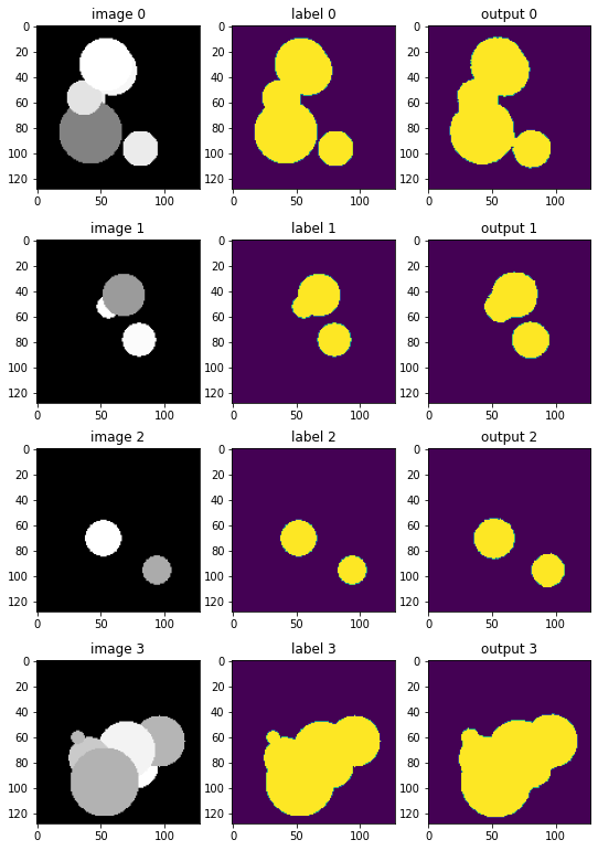
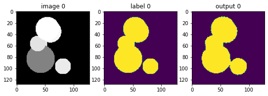
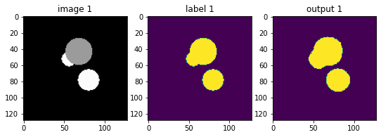
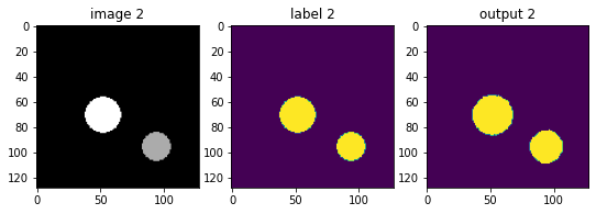
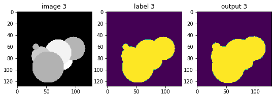
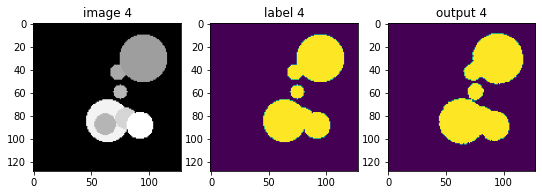
ベストモデル・パフォーマンス可視化


for i, valid_output in enumerate(runner.predict_loader(loader=val_loader)):
    if i > 4:
        break
    plt.figure("check", (9, 3))
    plt.subplot(1, 3, 1)
    plt.title("image " + str(i))
    plt.imshow(valid_output["img"].detach().cpu()[0, 0, :, :, 48], cmap="gray")
    plt.subplot(1, 3, 2)
    plt.title("label " + str(i))
    plt.imshow(valid_output["seg"].detach().cpu()[0, 0, :, :, 48])
    plt.subplot(1, 3, 3)
    plt.title("output " + str(i))
    logits = valid_output["logits"]
    plt.imshow((logits[0] > 0.5).float().detach().cpu()[0, :, :, 48])
    plt.show()

データディレクトリのクリーンアップ

Remove directory if a temporary was used.

if directory is None:
    shutil.rmtree(root_dir)

以上

MONAI 0.7 : tutorials : モジュール – 医用画像のロード

10/21/2021

MONAI 0.7 : tutorials : モジュール – 医用画像のロード (翻訳/解説)

翻訳 : (株)クラスキャットセールスインフォメーション
作成日時 : 10/21/2021 (0.7.0)

* 本ページは、MONAI の以下のドキュメントを翻訳した上で適宜、補足説明したものです：

Load medical images

クラスキャット人工知能研究開発支援サービス ★ 無料 Web セミナー開催中 ★

◆ クラスキャットは人工知能・テレワークに関する各種サービスを提供しております。お気軽にご相談ください :

人工知能研究開発支援
1. 人工知能研修サービス(経営者層向けオンサイト研修)
2. テクニカルコンサルティングサービス
3. 実証実験(プロトタイプ構築)
4. アプリケーションへの実装
人工知能研修サービス
PoC(概念実証)を失敗させないための支援
テレワーク & オンライン授業を支援

◆ 人工知能とビジネスをテーマに WEB セミナーを定期的に開催しています。スケジュール。

お住まいの地域に関係なく Web ブラウザからご参加頂けます。事前登録 が必要ですのでご注意ください。
ウェビナー運用には弊社製品「ClassCat® Webinar」を利用しています。

◆ お問合せ : 本件に関するお問い合わせ先は下記までお願いいたします。

株式会社クラスキャット セールス・マーケティング本部セールス・インフォメーション

E-Mail：sales-info@classcat.com ; WebSite: https://www.classcat.com/ ; Facebook

MONAI 0.7 : tutorials : モジュール – 医用画像のロード

このノートブックは MONAI で医用画像の様々な形式を簡単にロードして多くの追加の操作を実行する方法を紹介します。

このノートブックは MONAI で医用画像の様々な形式を簡単にロードして多くの追加の操作を実行する方法を説明します。

環境のセットアップ

!python -c "import monai" || pip install -q "monai-weekly[itk, pillow]"

インポートのセットアップ

# Copyright 2020 MONAI Consortium
# Licensed under the Apache License, Version 2.0 (the "License");
# you may not use this file except in compliance with the License.
# You may obtain a copy of the License at
#     http://www.apache.org/licenses/LICENSE-2.0
# Unless required by applicable law or agreed to in writing, software
# distributed under the License is distributed on an "AS IS" BASIS,
# WITHOUT WARRANTIES OR CONDITIONS OF ANY KIND, either express or implied.
# See the License for the specific language governing permissions and
# limitations under the License.

# Copyright 2020 MONAI Consortium
# Licensed under the Apache License, Version 2.0 (the "License");
# you may not use this file except in compliance with the License.
# You may obtain a copy of the License at
#     http://www.apache.org/licenses/LICENSE-2.0
# Unless required by applicable law or agreed to in writing, software
# distributed under the License is distributed on an "AS IS" BASIS,
# WITHOUT WARRANTIES OR CONDITIONS OF ANY KIND, either express or implied.
# See the License for the specific language governing permissions and
# limitations under the License.

import os
import shutil
import numpy as np
import itk
from PIL import Image
import tempfile
from monai.data import ITKReader, PILReader
from monai.transforms import (
    LoadImage, LoadImaged, EnsureChannelFirstd,
    Resized, EnsureTyped, Compose
)
from monai.config import print_config

print_config()

MONAI version: 0.6.0+22.g027947bf.dirty
Numpy version: 1.21.0
Pytorch version: 1.9.0
MONAI flags: HAS_EXT = False, USE_COMPILED = False
MONAI rev id: 027947bf91ff0dfac94f472ed1855cd49e3feb8d

Optional dependencies:
Pytorch Ignite version: 0.4.5
Nibabel version: 3.2.1
scikit-image version: 0.18.2
Pillow version: 8.2.0
Tensorboard version: 2.4.1
gdown version: 3.13.0
TorchVision version: 0.10.0
tqdm version: 4.61.1
lmdb version: 1.2.1
psutil version: 5.8.0
pandas version: 1.1.5
einops version: 0.3.0

For details about installing the optional dependencies, please visit:
    https://docs.monai.io/en/latest/installation.html#installing-the-recommended-dependencies

デフォルトの画像リーダーで Nifti 画像をロードする

MONAI はサポートされる suffix と下の順序に基づいてリーダーを自動的に選択します :

このローダを呼び出すとき実行時にユーザ指定されたリーダー。
リストの最新のものから最初のものへ登録されたリーダー。
デフォルトのリーダー : (nii, nii.gz -> NibabelReader), (png, jpg, bmp -> PILReader), (npz, npy -> NumpyReader), (others -> ITKReader).

サンプル画像を生成する

# generate 3D test images
tempdir = tempfile.mkdtemp()
test_image = np.random.rand(64, 128, 96)
filename = os.path.join(tempdir, "test_image.nii.gz")
itk_np_view = itk.image_view_from_array(test_image)
itk.imwrite(itk_np_view, filename)

画像ファイルをロードする

data, meta = LoadImage()(filename)
print(f"image data shape:{data.shape}")
print(f"meta data:{meta}")

image data shape:(96, 128, 64)
meta data:{'sizeof_hdr': array(348, dtype=int32), 'extents': array(0, dtype=int32), 'session_error': array(0, dtype=int16), 'dim_info': array(0, dtype=uint8), 'dim': array([  3,  96, 128,  64,   1,   1,   1,   1], dtype=int16), 'intent_p1': array(0., dtype=float32), 'intent_p2': array(0., dtype=float32), 'intent_p3': array(0., dtype=float32), 'intent_code': array(0, dtype=int16), 'datatype': array(64, dtype=int16), 'bitpix': array(64, dtype=int16), 'slice_start': array(0, dtype=int16), 'pixdim': array([1., 1., 1., 1., 0., 0., 0., 0.], dtype=float32), 'vox_offset': array(0., dtype=float32), 'scl_slope': array(nan, dtype=float32), 'scl_inter': array(nan, dtype=float32), 'slice_end': array(0, dtype=int16), 'slice_code': array(0, dtype=uint8), 'xyzt_units': array(2, dtype=uint8), 'cal_max': array(0., dtype=float32), 'cal_min': array(0., dtype=float32), 'slice_duration': array(0., dtype=float32), 'toffset': array(0., dtype=float32), 'glmax': array(0, dtype=int32), 'glmin': array(0, dtype=int32), 'qform_code': array(1, dtype=int16), 'sform_code': array(1, dtype=int16), 'quatern_b': array(0., dtype=float32), 'quatern_c': array(0., dtype=float32), 'quatern_d': array(1., dtype=float32), 'qoffset_x': array(-0., dtype=float32), 'qoffset_y': array(-0., dtype=float32), 'qoffset_z': array(0., dtype=float32), 'srow_x': array([-1.,  0.,  0., -0.], dtype=float32), 'srow_y': array([ 0., -1.,  0., -0.], dtype=float32), 'srow_z': array([0., 0., 1., 0.], dtype=float32), 'affine': array([[-1.,  0.,  0., -0.],
       [ 0., -1.,  0., -0.],
       [ 0.,  0.,  1.,  0.],
       [ 0.,  0.,  0.,  1.]]), 'original_affine': array([[-1.,  0.,  0., -0.],
       [ 0., -1.,  0., -0.],
       [ 0.,  0.,  1.,  0.],
       [ 0.,  0.,  0.,  1.]]), 'as_closest_canonical': False, 'spatial_shape': array([ 96, 128,  64], dtype=int16), 'original_channel_dim': 'no_channel', 'filename_or_obj': '/var/folders/6f/fdkl7m0x7sz3nj_t7p3ccgz00000gp/T/tmpq2arvyex/test_image.nii.gz'}

Nifti 画像のリストをロードしてそれらをマルチチャネル画像としてスタックする

ファイルのリストをロードし、それらを一緒にスタックして最初の次元として新しい次元を追加します。

そしてスタックされた結果を表わすために最初の画像のメタデータを使用します。

幾つかの画像サンプルを生成する

filenames = ["test_image.nii.gz", "test_image2.nii.gz", "test_image3.nii.gz"]
for i, name in enumerate(filenames):
    filenames[i] = os.path.join(tempdir, name)
    itk_np_view = itk.image_view_from_array(test_image)
    itk.imwrite(itk_np_view, filenames[i])

画像をロードする

出力データ shape は (3, 96, 128, 64) であることに注意してください、3 チャネル画像を示しています。

data, meta = LoadImage()(filenames)

print(f"image data shape:{data.shape}")
print(f"meta data:{meta}")

image data shape:(3, 96, 128, 64)
meta data:{'sizeof_hdr': array(348, dtype=int32), 'extents': array(0, dtype=int32), 'session_error': array(0, dtype=int16), 'dim_info': array(0, dtype=uint8), 'dim': array([  3,  96, 128,  64,   1,   1,   1,   1], dtype=int16), 'intent_p1': array(0., dtype=float32), 'intent_p2': array(0., dtype=float32), 'intent_p3': array(0., dtype=float32), 'intent_code': array(0, dtype=int16), 'datatype': array(64, dtype=int16), 'bitpix': array(64, dtype=int16), 'slice_start': array(0, dtype=int16), 'pixdim': array([1., 1., 1., 1., 0., 0., 0., 0.], dtype=float32), 'vox_offset': array(0., dtype=float32), 'scl_slope': array(nan, dtype=float32), 'scl_inter': array(nan, dtype=float32), 'slice_end': array(0, dtype=int16), 'slice_code': array(0, dtype=uint8), 'xyzt_units': array(2, dtype=uint8), 'cal_max': array(0., dtype=float32), 'cal_min': array(0., dtype=float32), 'slice_duration': array(0., dtype=float32), 'toffset': array(0., dtype=float32), 'glmax': array(0, dtype=int32), 'glmin': array(0, dtype=int32), 'qform_code': array(1, dtype=int16), 'sform_code': array(1, dtype=int16), 'quatern_b': array(0., dtype=float32), 'quatern_c': array(0., dtype=float32), 'quatern_d': array(1., dtype=float32), 'qoffset_x': array(-0., dtype=float32), 'qoffset_y': array(-0., dtype=float32), 'qoffset_z': array(0., dtype=float32), 'srow_x': array([-1.,  0.,  0., -0.], dtype=float32), 'srow_y': array([ 0., -1.,  0., -0.], dtype=float32), 'srow_z': array([0., 0., 1., 0.], dtype=float32), 'affine': array([[-1.,  0.,  0., -0.],
       [ 0., -1.,  0., -0.],
       [ 0.,  0.,  1.,  0.],
       [ 0.,  0.,  0.,  1.]]), 'original_affine': array([[-1.,  0.,  0., -0.],
       [ 0., -1.,  0., -0.],
       [ 0.,  0.,  1.,  0.],
       [ 0.,  0.,  0.,  1.]]), 'as_closest_canonical': False, 'spatial_shape': array([ 96, 128,  64], dtype=int16), 'original_channel_dim': 0, 'filename_or_obj': '/var/folders/6f/fdkl7m0x7sz3nj_t7p3ccgz00000gp/T/tmpq2arvyex/test_image.nii.gz'}

DICOM 形式の 3D 画像のロード

サンプル画像を生成する

filename = os.path.join(tempdir, "test_image.dcm")
dcm_image = np.random.randint(256, size=(64, 128, 96)).astype(np.uint8)
itk_np_view = itk.image_view_from_array(dcm_image)
itk.imwrite(itk_np_view, filename)

Ref.

!pip install pydicom

from pydicom import dcmread
from pydicom.data import get_testdata_file

ds = dcmread(filename)
 print(type(ds.PixelData), len(ds.PixelData), ds.PixelData[:2])

<class 'bytes'> 786432 b'\x97\xb3'

arr = ds.pixel_array
print(type(arr), arr.shape, arr.dtype)

<class 'numpy.ndarray'> (64, 128, 96) uint8

plt.imshow(arr[:,:,0])

画像のロード

data, meta = LoadImage()(filename)

print(f"image data shape:{data.shape}")
print(f"meta data:{meta}")

image data shape:(96, 128, 64)
meta data:{'0008|0016': '1.2.840.10008.5.1.4.1.1.7.2', '0008|0018': '1.2.826.0.1.3680043.2.1125.1.49144329026051408197861589261117151', '0008|0020': '20210722', '0008|0030': '170636.794924 ', '0008|0050': '', '0008|0060': 'OT', '0008|0090': '', '0010|0010': '', '0010|0020': '', '0010|0030': '', '0010|0040': '', '0020|000d': '1.2.826.0.1.3680043.2.1125.1.55082693700512159103862591206822067', '0020|000e': '1.2.826.0.1.3680043.2.1125.1.88286845929415088271370520342732963', '0020|0010': '', '0020|0011': '', '0020|0013': '', '0020|0052': '1.2.826.0.1.3680043.2.1125.1.54872246537810654209027218359324264', '0028|0002': '1', '0028|0004': 'MONOCHROME2 ', '0028|0008': '64', '0028|0009': '(5200,9230)', '0028|0010': '128', '0028|0011': '96', '0028|0100': '8', '0028|0101': '8', '0028|0102': '7', '0028|0103': '0', '0028|1052': '0 ', '0028|1053': '1 ', '0028|1054': 'US', 'spacing': array([1., 1., 1.]), 'original_affine': array([[-1.,  0.,  0.,  0.],
       [ 0., -1.,  0.,  0.],
       [ 0.,  0.,  1.,  0.],
       [ 0.,  0.,  0.,  1.]]), 'affine': array([[-1.,  0.,  0.,  0.],
       [ 0., -1.,  0.,  0.],
       [ 0.,  0.,  1.,  0.],
       [ 0.,  0.,  0.,  1.]]), 'spatial_shape': array([ 96, 128,  64]), 'original_channel_dim': 'no_channel', 'filename_or_obj': '/var/folders/6f/fdkl7m0x7sz3nj_t7p3ccgz00000gp/T/tmpq2arvyex/test_image.dcm'}

DICOM 画像のリストをロードしてそれらをマルチチャネル画像としてスタックする

ファイルのリストをロードし、それらを一緒にスタックして最初の次元として新しい次元を追加します。

そしてスタックされた結果を表わすために最初の画像のメタデータを使用します。

幾つかの画像サンプルを生成する

filenames = ["test_image-1.dcm", "test_image-2.dcm", "test_image-3.dcm"]
for i, name in enumerate(filenames):
    filenames[i] = os.path.join(tempdir, name)
    dcm_image = np.random.randint(256, size=(64, 128, 96)).astype(np.uint8)
    itk_np_view = itk.image_view_from_array(dcm_image)
    itk.imwrite(itk_np_view, filenames[i])

画像をロードする

data, meta = LoadImage()(filenames)

print(f"image data shape:{data.shape}")
print(f"meta data:{meta}")

image data shape:(3, 96, 128, 64)
meta data:{'0008|0016': '1.2.840.10008.5.1.4.1.1.7.2', '0008|0018': '1.2.826.0.1.3680043.2.1125.1.70459687821230247148357643462536357', '0008|0020': '20210722', '0008|0030': '170636.830318 ', '0008|0050': '', '0008|0060': 'OT', '0008|0090': '', '0010|0010': '', '0010|0020': '', '0010|0030': '', '0010|0040': '', '0020|000d': '1.2.826.0.1.3680043.2.1125.1.29026801319907695346385092515779097', '0020|000e': '1.2.826.0.1.3680043.2.1125.1.48166663359438709592920991059259631', '0020|0010': '', '0020|0011': '', '0020|0013': '', '0020|0052': '1.2.826.0.1.3680043.2.1125.1.52318595437965660783667062205792724', '0028|0002': '1', '0028|0004': 'MONOCHROME2 ', '0028|0008': '64', '0028|0009': '(5200,9230)', '0028|0010': '128', '0028|0011': '96', '0028|0100': '8', '0028|0101': '8', '0028|0102': '7', '0028|0103': '0', '0028|1052': '0 ', '0028|1053': '1 ', '0028|1054': 'US', 'spacing': array([1., 1., 1.]), 'original_affine': array([[-1.,  0.,  0.,  0.],
       [ 0., -1.,  0.,  0.],
       [ 0.,  0.,  1.,  0.],
       [ 0.,  0.,  0.,  1.]]), 'affine': array([[-1.,  0.,  0.,  0.],
       [ 0., -1.,  0.,  0.],
       [ 0.,  0.,  1.,  0.],
       [ 0.,  0.,  0.,  1.]]), 'spatial_shape': array([ 96, 128,  64]), 'original_channel_dim': 0, 'filename_or_obj': '/var/folders/6f/fdkl7m0x7sz3nj_t7p3ccgz00000gp/T/tmpq2arvyex/test_image-1.dcm'}

PNG 形式で 2D 画像をロードする

画像を生成する

test_image = np.random.randint(0, 256, size=[128, 256])
filename = os.path.join(tempdir, "test_image.png")
Image.fromarray(test_image.astype("uint8")).save(filename)

画像をロードする

data, meta = LoadImage()(filename)

print(f"image data shape:{data.shape}")
print(f"meta data:{meta}")

image data shape:(256, 128)
meta data:{'format': 'PNG', 'mode': 'L', 'width': 256, 'height': 128, 'spatial_shape': array([256, 128]), 'original_channel_dim': 'no_channel', 'filename_or_obj': '/var/folders/6f/fdkl7m0x7sz3nj_t7p3ccgz00000gp/T/tmpq2arvyex/test_image.png'}

指定した画像リーダで画像をロードする

そして画像リーダーのための追加パラメータを設定できます、例えば、ITKReader のために c_order_axis_indexing=True を設定すると、このパラメータは後で ITK read() 関数に渡されます。

loader = LoadImage()
loader.register(ITKReader())
data, meta = loader(filename)

print(f"image data shape:{data.shape}")
print(f"meta data:{meta}")

image data shape:(256, 128)
meta data:{'spacing': array([1., 1.]), 'original_affine': array([[-1.,  0.,  0.],
       [ 0., -1.,  0.],
       [ 0.,  0.,  1.]]), 'affine': array([[-1.,  0.,  0.],
       [ 0., -1.,  0.],
       [ 0.,  0.,  1.]]), 'spatial_shape': array([256, 128]), 'original_channel_dim': 'no_channel', 'filename_or_obj': '/var/folders/6f/fdkl7m0x7sz3nj_t7p3ccgz00000gp/T/tmpq2arvyex/test_image.png'}

画像をロードして追加の操作を実行する

幾つかの画像リーダーはファイルから画像を読んだ後の追加の操作をサポートできます。

例えば、PILReader のためにコンバータを設定できます : PILReader(converter=lambda image: image.convert(“LA”))

loader = LoadImage(PILReader(converter=lambda image: image.convert("LA")))
data, meta = loader(filename)

print(f"image data shape:{data.shape}")
print(f"meta data:{meta}")

image data shape:(256, 128, 2)
meta data:{'format': None, 'mode': 'LA', 'width': 256, 'height': 128, 'spatial_shape': array([256, 128]), 'original_channel_dim': -1, 'filename_or_obj': '/var/folders/6f/fdkl7m0x7sz3nj_t7p3ccgz00000gp/T/tmpq2arvyex/test_image.png'}

LoadImage を他の変換と組み合わせる

変換チェインを構築するために LoadImage を他の変換と接続することは非常に簡単です。

transform = Compose([
    LoadImaged(keys="image"),
    EnsureChannelFirstd(keys="image"),
    Resized(keys="image", spatial_size=[64, 64]),
    EnsureTyped("image"),
])
test_data = {"image": filename}
result = transform(test_data)
print(f"image data shape:{result['image'].shape}")
print(f"meta data:{result['image_meta_dict']}")

image data shape:torch.Size([1, 64, 64])
meta data:{'format': 'PNG', 'mode': 'L', 'width': 256, 'height': 128, 'spatial_shape': array([256, 128]), 'original_channel_dim': 'no_channel', 'filename_or_obj': '/var/folders/6f/fdkl7m0x7sz3nj_t7p3ccgz00000gp/T/tmpq2arvyex/test_image.png'}

データディレクトリのクリーンアップ

一時ディレクトリが使用された場合にはディレクトリを削除します。

shutil.rmtree(tempdir)

以上

MONAI 0.7 : tutorials : モジュール – Nifti 読み込み例

10/21/2021

MONAI 0.7 : tutorials : モジュール – Nifti 読み込み例 (翻訳/解説)

翻訳 : (株)クラスキャットセールスインフォメーション
作成日時 : 10/21/2021 (0.7.0)

* 本ページは、MONAI の以下のドキュメントを翻訳した上で適宜、補足説明したものです：

Nifti Read Example

クラスキャット人工知能研究開発支援サービス ★ 無料 Web セミナー開催中 ★

◆ クラスキャットは人工知能・テレワークに関する各種サービスを提供しております。お気軽にご相談ください :

人工知能研究開発支援
1. 人工知能研修サービス(経営者層向けオンサイト研修)
2. テクニカルコンサルティングサービス
3. 実証実験(プロトタイプ構築)
4. アプリケーションへの実装
人工知能研修サービス
PoC(概念実証)を失敗させないための支援
テレワーク & オンライン授業を支援

◆ 人工知能とビジネスをテーマに WEB セミナーを定期的に開催しています。スケジュール。

お住まいの地域に関係なく Web ブラウザからご参加頂けます。事前登録 が必要ですのでご注意ください。
ウェビナー運用には弊社製品「ClassCat® Webinar」を利用しています。

◆ お問合せ : 本件に関するお問い合わせ先は下記までお願いいたします。

株式会社クラスキャット セールス・マーケティング本部セールス・インフォメーション

E-Mail：sales-info@classcat.com ; WebSite: https://www.classcat.com/ ; Facebook

MONAI 0.7 : tutorials : モジュール – Nifti 読み込み例

NIfTI ファイルを読みそしてそれらからロードされたボリュームの画像パッチに渡る反復を例示して説明します。

このノートブックの目的は、NIfTI ファイルを読みそしてそれらからロードされたボリュームの画像パッチに渡る反復を例示して説明します。

環境のセットアップ

!python -c "import monai" || pip install -q "monai-weekly[nibabel]"

インポートのセットアップ

# Copyright 2020 MONAI Consortium
# Licensed under the Apache License, Version 2.0 (the "License");
# you may not use this file except in compliance with the License.
# You may obtain a copy of the License at
#     http://www.apache.org/licenses/LICENSE-2.0
# Unless required by applicable law or agreed to in writing, software
# distributed under the License is distributed on an "AS IS" BASIS,
# WITHOUT WARRANTIES OR CONDITIONS OF ANY KIND, either express or implied.
# See the License for the specific language governing permissions and
# limitations under the License.

import glob
import os
import shutil
import tempfile

import nibabel as nib
import numpy as np
import torch

from monai.config import print_config
from monai.data import (
    ArrayDataset, GridPatchDataset, create_test_image_3d, PatchIter)
from monai.transforms import (
    AddChannel,
    Compose,
    LoadImage,
    RandSpatialCrop,
    ScaleIntensity,
    EnsureType,
)
from monai.utils import first

print_config()

MONAI version: 0.6.0rc1+23.gc6793fd0
Numpy version: 1.20.3
Pytorch version: 1.9.0a0+c3d40fd
MONAI flags: HAS_EXT = True, USE_COMPILED = False
MONAI rev id: c6793fd0f316a448778d0047664aaf8c1895fe1c

Optional dependencies:
Pytorch Ignite version: 0.4.5
Nibabel version: 3.2.1
scikit-image version: 0.15.0
Pillow version: 7.0.0
Tensorboard version: 2.5.0
gdown version: 3.13.0
TorchVision version: 0.10.0a0
ITK version: 5.1.2
tqdm version: 4.53.0
lmdb version: 1.2.1
psutil version: 5.8.0
pandas version: 1.1.4
einops version: 0.3.0

For details about installing the optional dependencies, please visit:
    https://docs.monai.io/en/latest/installation.html#installing-the-recommended-dependencies

データディレクトリのセットアップ

directory = os.environ.get("MONAI_DATA_DIRECTORY")
root_dir = tempfile.mkdtemp() if directory is None else directory
print(root_dir)

/tmp/tmp3y4h4i5o

幾つかのテスト Nifti ファイルを作成します :

for i in range(5):
    im, seg = create_test_image_3d(128, 128, 128)

    n = nib.Nifti1Image(im, np.eye(4))
    nib.save(n, os.path.join(root_dir, f"im{i}.nii.gz"))

    n = nib.Nifti1Image(seg, np.eye(4))
    nib.save(n, os.path.join(root_dir, f"seg{i}.nii.gz"))

Ref.

test_file = root_dir + "/im0.nii.gz" 
img_test = nib.load(test_file)
print(type(img_test), img_test.shape)

img_ary = img_test.get_fdata()[:, :, 64]
print(type(img_ary), img_ary.shape, img_ary.dtype)

plt.imshow(img_ary)

<class 'nibabel.nifti1.Nifti1Image'> (128, 128, 128)
<class 'numpy.ndarray'> (128, 128) float64

plt.subplots(4, 3, figsize=(128, 128))
for i in range(12):
    img_ary = img_test.get_fdata()[:, :, i*10]
    plt.subplot(4, 3, i + 1)
    plt.imshow(img_ary, cmap="gray")
plt.tight_layout()
plt.show()

ロードされた Nifti ファイルから一様なランダムパッチを生成するデータローダを作成します :

images = sorted(glob.glob(os.path.join(root_dir, "im*.nii.gz")))
segs = sorted(glob.glob(os.path.join(root_dir, "seg*.nii.gz")))

imtrans = Compose(
    [
        LoadImage(image_only=True),
        ScaleIntensity(),
        AddChannel(),
        RandSpatialCrop((64, 64, 64), random_size=False),
        EnsureType(),
    ]
)

segtrans = Compose(
    [
        LoadImage(image_only=True),
        AddChannel(),
        RandSpatialCrop((64, 64, 64), random_size=False),
        EnsureType(),
    ]
)

ds = ArrayDataset(images, imtrans, segs, segtrans)

loader = torch.utils.data.DataLoader(
    ds, batch_size=10, num_workers=2, pin_memory=torch.cuda.is_available()
)
im, seg = first(loader)
print(im.shape, seg.shape)

torch.Size([5, 1, 64, 64, 64]) torch.Size([5, 1, 64, 64, 64])

あるいは、ロードされた画像から規則的なグリッド順でパッチを生成するデータローダを作成します :

imtrans = Compose([LoadImage(image_only=True),
                   ScaleIntensity(), AddChannel(), EnsureType()])

segtrans = Compose([LoadImage(image_only=True), AddChannel(), EnsureType()])

ds = ArrayDataset(images, imtrans, segs, segtrans)
patch_iter = PatchIter(patch_size=(64, 64, 64), start_pos=(0, 0, 0))


def img_seg_iter(x):
    return (zip(patch_iter(x[0]), patch_iter(x[1])),)


ds = GridPatchDataset(ds, img_seg_iter, with_coordinates=False)

loader = torch.utils.data.DataLoader(
    ds, batch_size=10, num_workers=2, pin_memory=torch.cuda.is_available()
)
im, seg = first(loader)
print("image shapes:", im[0].shape, seg[0].shape)
print("coordinates shapes:", im[1].shape, seg[1].shape)

image shapes: torch.Size([3, 1, 64, 64, 64]) torch.Size([3, 1, 64, 64, 64])
coordinates shapes: torch.Size([3, 4, 2]) torch.Size([3, 4, 2])

データディレクトリのクリーンアップ

一時ディレクトリが使用された場合にはディレクトリを削除します。

if directory is None:
    shutil.rmtree(root_dir)

以上

MONAI 0.7 : tutorials : モジュール – ImageDataset

10/20/2021

MONAI 0.7 : tutorials : モジュール – ImageDataset (翻訳/解説)

翻訳 : (株)クラスキャットセールスインフォメーション
作成日時 : 10/20/2021 (0.7.0)

* 本ページは、MONAI の以下のドキュメントを翻訳した上で適宜、補足説明したものです：

ImageDataset

クラスキャット人工知能研究開発支援サービス ★ 無料 Web セミナー開催中 ★

◆ クラスキャットは人工知能・テレワークに関する各種サービスを提供しております。お気軽にご相談ください :

人工知能研究開発支援
1. 人工知能研修サービス(経営者層向けオンサイト研修)
2. テクニカルコンサルティングサービス
3. 実証実験(プロトタイプ構築)
4. アプリケーションへの実装
人工知能研修サービス
PoC(概念実証)を失敗させないための支援
テレワーク & オンライン授業を支援

◆ 人工知能とビジネスをテーマに WEB セミナーを定期的に開催しています。スケジュール。

お住まいの地域に関係なく Web ブラウザからご参加頂けます。事前登録 が必要ですのでご注意ください。
ウェビナー運用には弊社製品「ClassCat® Webinar」を利用しています。

◆ お問合せ : 本件に関するお問い合わせ先は下記までお願いいたします。

株式会社クラスキャット セールス・マーケティング本部セールス・インフォメーション

E-Mail：sales-info@classcat.com ; WebSite: https://www.classcat.com/ ; Facebook

MONAI 0.7 : tutorials : モジュール – ImageDataset

ノートブックは monai.data.ImageDataset モジュールの基本的な使い方を紹介します。

このノートブックは monai.data.ImageDataset の基本的な使い方を紹介します。

環境のセットアップ

!python -c "import monai" || pip install -q "monai-weekly[itk, pillow]"

インポートのセットアップ

# Copyright 2020 - 2021 MONAI Consortium
# Licensed under the Apache License, Version 2.0 (the "License");
# you may not use this file except in compliance with the License.
# You may obtain a copy of the License at
#     http://www.apache.org/licenses/LICENSE-2.0
# Unless required by applicable law or agreed to in writing, software
# distributed under the License is distributed on an "AS IS" BASIS,
# WITHOUT WARRANTIES OR CONDITIONS OF ANY KIND, either express or implied.
# See the License for the specific language governing permissions and
# limitations under the License.

# Copyright 2020 MONAI Consortium
# Licensed under the Apache License, Version 2.0 (the "License");
# you may not use this file except in compliance with the License.
# You may obtain a copy of the License at
#     http://www.apache.org/licenses/LICENSE-2.0
# Unless required by applicable law or agreed to in writing, software
# distributed under the License is distributed on an "AS IS" BASIS,
# WITHOUT WARRANTIES OR CONDITIONS OF ANY KIND, either express or implied.
# See the License for the specific language governing permissions and
# limitations under the License.
import os
import tempfile
import shutil

import nibabel as nib
import numpy as np

from monai.data import ImageDataset
from monai.transforms import Compose, EnsureChannelFirst, RandAdjustContrast, Spacing
from monai.config import print_config

print_config()

MONAI version: 0.6.0rc1+23.gc6793fd0
Numpy version: 1.20.3
Pytorch version: 1.9.0a0+c3d40fd
MONAI flags: HAS_EXT = True, USE_COMPILED = False
MONAI rev id: c6793fd0f316a448778d0047664aaf8c1895fe1c

Optional dependencies:
Pytorch Ignite version: 0.4.5
Nibabel version: 3.2.1
scikit-image version: 0.15.0
Pillow version: 8.2.0
Tensorboard version: 2.5.0
gdown version: 3.13.0
TorchVision version: 0.10.0a0
ITK version: 5.1.2
tqdm version: 4.53.0
lmdb version: 1.2.1
psutil version: 5.8.0
pandas version: 1.1.4
einops version: 0.3.0

For details about installing the optional dependencies, please visit:
    https://docs.monai.io/en/latest/installation.html#installing-the-recommended-dependencies

# Generate some image data
tempdir = tempfile.mkdtemp()
img_ = nib.Nifti1Image(np.random.randint(0, 2, size=(20, 20, 20)), np.eye(4))
seg_ = nib.Nifti1Image(np.random.randint(0, 2, size=(20, 20, 20)), np.eye(4))
img_name = os.path.join(tempdir, "img.nii.gz")
seg_name = os.path.join(tempdir, "seg.nii.gz")
nib.save(img_, img_name)
nib.save(seg_, seg_name)
img_list = [img_name]
seg_list = [seg_name]

変換のカスタマイズされたチェインを構築する

TestCompose は前処理パイプラインの一部として追加のメタデータを処理するために使用されます。

class TestCompose(Compose):
    def __call__(self, data, meta):
        data = self.transforms[0](data, meta)  # ensure channel first
        data, _, meta["affine"] = self.transforms[1](data, meta["affine"])  # spacing
        if len(self.transforms) == 3:
            return self.transforms[2](data), meta  # image contrast
        return data, meta


img_xform = TestCompose([EnsureChannelFirst(), Spacing(pixdim=(1.5, 1.5, 3.0)), RandAdjustContrast()])
seg_xform = TestCompose([EnsureChannelFirst(), Spacing(pixdim=(1.5, 1.5, 3.0), mode="nearest")])
img_dataset = ImageDataset(
    image_files=img_list,
    seg_files=seg_list,
    transform=img_xform,
    seg_transform=seg_xform,
    image_only=False,
    transform_with_metadata=True,
)
print("image shape:", img_dataset[0][0].shape)
print("seg. shape:", img_dataset[0][1].shape)


image shape: (1, 14, 14, 7)
seg. shape: (1, 14, 14, 7)

ディレクトリのクリーンアップ

shutil.rmtree(tempdir)

以上

MONAI 0.7 : tutorials : モジュール – CSV データセットで CSV ファイルのロード

10/20/2021

MONAI 0.7 : tutorials : モジュール – CSV データセットで CSV ファイルのロード (翻訳/解説)

翻訳 : (株)クラスキャットセールスインフォメーション
作成日時 : 10/20/2021 (0.7.0)

* 本ページは、MONAI の以下のドキュメントを翻訳した上で適宜、補足説明したものです：

Load CSV files with CSV Datasets

MONAI 0.7 : tutorials : モジュール – CSV データセットで CSV ファイルのロード

チュートリアルは CSVDataset と CSVIterableDataset の使い方を示し、複数の CSV ファイルをロードして後処理ロジックを実行します。

このチュートリアルは CSVDataset と CSVIterableDataset モジュールに基づいて CSV ファイルからデータをロードする方法を示します。そしてデータ上で後処理ロジックを実行します。

環境のセットアップ

!python -c "import monai" || pip install -q "monai-weekly[pandas, pillow]"
%matplotlib inline

インポートのセットアップ

# Copyright 2020 MONAI Consortium
# Licensed under the Apache License, Version 2.0 (the "License");
# you may not use this file except in compliance with the License.
# You may obtain a copy of the License at
#     http://www.apache.org/licenses/LICENSE-2.0
# Unless required by applicable law or agreed to in writing, software
# distributed under the License is distributed on an "AS IS" BASIS,
# WITHOUT WARRANTIES OR CONDITIONS OF ANY KIND, either express or implied.
# See the License for the specific language governing permissions and
# limitations under the License.

import os
import tempfile
import shutil
import sys
import matplotlib.pyplot as plt
import pandas as pd
import PIL
import numpy as np

from monai.data import CSVDataset, CSVIterableDataset, DataLoader
from monai.apps import download_and_extract
from monai.config import print_config
from monai.transforms import Compose, LoadImaged, ToNumpyd
from monai.utils import first

print_config()

MONAI version: 0.6.0rc1+23.gc6793fd0
Numpy version: 1.20.3
Pytorch version: 1.9.0a0+c3d40fd
MONAI flags: HAS_EXT = True, USE_COMPILED = False
MONAI rev id: c6793fd0f316a448778d0047664aaf8c1895fe1c

Optional dependencies:
Pytorch Ignite version: 0.4.5
Nibabel version: 3.2.1
scikit-image version: 0.15.0
Pillow version: 8.2.0
Tensorboard version: 2.5.0
gdown version: 3.13.0
TorchVision version: 0.10.0a0
ITK version: 5.1.2
tqdm version: 4.53.0
lmdb version: 1.2.1
psutil version: 5.8.0
pandas version: 1.1.4
einops version: 0.3.0

For details about installing the optional dependencies, please visit:
    https://docs.monai.io/en/latest/installation.html#installing-the-recommended-dependencies

データディレクトリのセットアップ

directory = os.environ.get("MONAI_DATA_DIRECTORY")
root_dir = tempfile.mkdtemp() if directory is None else directory
print(root_dir)

/workspace/data/medical

データセットをダウンロードする

ここではデモで MedNIST データセットの幾つかの画像を使用します。データセットをダウンロードして展開してください。

MedMNIST データセットは TCIA, RSNA Bone Age チャレンジと NIH Chest X-ray データセットからの様々なセットから集められました。

データセットは Dr. Bradley J. Erickson M.D., Ph.D. (Department of Radiology, Mayo Clinic) のお陰により Creative Commons CC BY-SA 4.0 ライセンスのもとで利用可能になっています。

resource = "https://drive.google.com/uc?id=1QsnnkvZyJPcbRoV_ArW8SnE1OTuoVbKE"
md5 = "0bc7306e7427e00ad1c5526a6677552d"

compressed_file = os.path.join(root_dir, "MedNIST.tar.gz")
data_dir = os.path.join(root_dir, "MedNIST")
if not os.path.exists(data_dir):
    download_and_extract(resource, compressed_file, root_dir, md5)

ハンド・カテゴリーの幾つかの医療画像をプロットする

plt.subplots(1, 5, figsize=(10, 10))
for i in range(5):
    filename = f"00000{i}.jpeg"
    im = PIL.Image.open(os.path.join(data_dir, "Hand", filename))
    arr = np.array(im)
    plt.subplot(3, 3, i + 1)
    plt.xlabel(filename)
    plt.imshow(arr, cmap="gray", vmin=0, vmax=255)
plt.tight_layout()
plt.show()

テストのために 3 CSV ファイルを生成する

ここで画像の特性をストアするために 3 CSV ファイルを生成します、欠損値を含みます。

test_data1 = [
    ["subject_id", "label", "image", "ehr_0", "ehr_1", "ehr_2"],
    ["s000000", 5, os.path.join(data_dir, "Hand", "000000.jpeg"), 2.007843256, 2.29019618, 2.054902077],
    ["s000001", 0, os.path.join(data_dir, "Hand", "000001.jpeg"), 6.839215755, 6.474509716, 5.862744808],
    ["s000002", 4, os.path.join(data_dir, "Hand", "000002.jpeg"), 3.772548914, 4.211764812, 4.635294437],
    ["s000003", 1, os.path.join(data_dir, "Hand", "000003.jpeg"), 3.333333254, 3.235294342, 3.400000095],
    ["s000004", 9, os.path.join(data_dir, "Hand", "000004.jpeg"), 6.427451134, 6.254901886, 5.976470947],
]
test_data2 = [
    ["subject_id", "ehr_3", "ehr_4", "ehr_5", "ehr_6", "ehr_7", "ehr_8"],
    ["s000000", 3.019608021, 3.807843208, 3.584313869, 3.141176462, 3.1960783, 4.211764812],
    ["s000001", 5.192157269, 5.274509907, 5.250980377, 4.647058964, 4.886274338, 4.392156601],
    ["s000002", 5.298039436, 9.545097351, 12.57254887, 6.799999714, 2.1960783, 1.882352948],
    ["s000003", 3.164705753, 3.086274624, 3.725490093, 3.698039293, 3.698039055, 3.701960802],
    ["s000004", 6.26274538, 7.717647076, 9.584313393, 6.082352638, 2.662744999, 2.34117651],
]
test_data3 = [
    ["subject_id", "ehr_9", "ehr_10", "meta_0", "meta_1", "meta_2"],
    ["s000000", 6.301961422, 6.470588684, "TRUE", "TRUE", "TRUE"],
    ["s000001", 5.219608307, 7.827450752, "FALSE", "TRUE", "FALSE"],
    ["s000002", 1.882352948, 2.031372547, "TRUE", "FALSE", "TRUE"],
    ["s000003", 3.309803963, 3.729412079, "FALSE", "FALSE", "TRUE"],
    ["s000004", 2.062745094, 2.34117651, "FALSE", "TRUE", "TRUE"],
    # generate missing values in the row
    ["s000005", 3.353655643, 1.675674543, "TRUE", "TRUE", "FALSE"],
]


def prepare_csv_file(data, filepath):
    with open(filepath, "w") as f:
        for d in data:
            f.write((",".join([str(i) for i in d])) + "\n")


filepath1 = os.path.join(data_dir, "test_data1.csv")
filepath2 = os.path.join(data_dir, "test_data2.csv")
filepath3 = os.path.join(data_dir, "test_data3.csv")
prepare_csv_file(test_data1, filepath1)
prepare_csv_file(test_data2, filepath2)
prepare_csv_file(test_data3, filepath3)

CSVDataset でシングル CSV ファイルをロードする

dataset = CSVDataset(filename=filepath1)
# construct pandas table to show the data, `CSVDataset` inherits from PyTorch Dataset
print(pd.DataFrame(dataset.data))

  subject_id  label                                             image  \
0    s000000      5  /workspace/data/medical/MedNIST/Hand/000000.jpeg   
1    s000001      0  /workspace/data/medical/MedNIST/Hand/000001.jpeg   
2    s000002      4  /workspace/data/medical/MedNIST/Hand/000002.jpeg   
3    s000003      1  /workspace/data/medical/MedNIST/Hand/000003.jpeg   
4    s000004      9  /workspace/data/medical/MedNIST/Hand/000004.jpeg   

      ehr_0     ehr_1     ehr_2  
0  2.007843  2.290196  2.054902  
1  6.839216  6.474510  5.862745  
2  3.772549  4.211765  4.635294  
3  3.333333  3.235294  3.400000  
4  6.427451  6.254902  5.976471

複数の CSV ファイルをロードしてテーブルを結合する

dataset = CSVDataset([filepath1, filepath2, filepath3], on="subject_id")
# construct pandas table to show the joined data of 3 tables
print(pd.DataFrame(dataset.data))

  subject_id  label                                             image  \
0    s000000      5  /workspace/data/medical/MedNIST/Hand/000000.jpeg   
1    s000001      0  /workspace/data/medical/MedNIST/Hand/000001.jpeg   
2    s000002      4  /workspace/data/medical/MedNIST/Hand/000002.jpeg   
3    s000003      1  /workspace/data/medical/MedNIST/Hand/000003.jpeg   
4    s000004      9  /workspace/data/medical/MedNIST/Hand/000004.jpeg   

      ehr_0     ehr_1     ehr_2     ehr_3     ehr_4      ehr_5     ehr_6  \
0  2.007843  2.290196  2.054902  3.019608  3.807843   3.584314  3.141176   
1  6.839216  6.474510  5.862745  5.192157  5.274510   5.250980  4.647059   
2  3.772549  4.211765  4.635294  5.298039  9.545097  12.572549  6.800000   
3  3.333333  3.235294  3.400000  3.164706  3.086275   3.725490  3.698039   
4  6.427451  6.254902  5.976471  6.262745  7.717647   9.584313  6.082353   

      ehr_7     ehr_8     ehr_9    ehr_10  meta_0  meta_1  meta_2  
0  3.196078  4.211765  6.301961  6.470589    True    True    True  
1  4.886274  4.392157  5.219608  7.827451   False    True   False  
2  2.196078  1.882353  1.882353  2.031373    True   False    True  
3  3.698039  3.701961  3.309804  3.729412   False   False    True  
4  2.662745  2.341177  2.062745  2.341177   False    True    True

3 CSV ファイルから選択された行と選択された列だけをロードする

ここでは rows: 0 – 1 と 3, columns: “subject_id”, “label”, “ehr_1”, “ehr_7”, “meta_1” をロードします。

dataset = CSVDataset(
    filename=[filepath1, filepath2, filepath3],
    row_indices=[[0, 2], 3],  # load row: 0, 1, 3
    col_names=["subject_id", "label", "ehr_1", "ehr_7", "meta_1"],
)
# construct pandas table to show the joined and selected data
print(pd.DataFrame(dataset.data))

  subject_id  label     ehr_1     ehr_7  meta_1
0    s000000      5  2.290196  3.196078    True
1    s000001      0  6.474510  4.886274    True
2    s000003      1  3.235294  3.698039   False

新しいカラムを生成するためにカラムをロードしてグループ分けする

ここでは 3 CSV ファイルをロードして新しい ehr カラムを生成するために総ての ehr_* カラムをグループ分けし、そして新しい meta カラムを生成するために総ての meta_* カラムをグループ分けします。


dataset = CSVDataset(
    filename=[filepath1, filepath2, filepath3],
    col_names=["subject_id", "image", *[f"ehr_{i}" for i in range(11)], "meta_0", "meta_1", "meta_2"],
    col_groups={"ehr": [f"ehr_{i}" for i in range(11)], "meta": ["meta_0", "meta_1", "meta_2"]},
)
# construct pandas table to show the joined, selected and generated data
print(pd.DataFrame(dataset.data))

  subject_id                                             image     ehr_0  \
0    s000000  /workspace/data/medical/MedNIST/Hand/000000.jpeg  2.007843   
1    s000001  /workspace/data/medical/MedNIST/Hand/000001.jpeg  6.839216   
2    s000002  /workspace/data/medical/MedNIST/Hand/000002.jpeg  3.772549   
3    s000003  /workspace/data/medical/MedNIST/Hand/000003.jpeg  3.333333   
4    s000004  /workspace/data/medical/MedNIST/Hand/000004.jpeg  6.427451   

      ehr_1     ehr_2     ehr_3     ehr_4      ehr_5     ehr_6     ehr_7  \
0  2.290196  2.054902  3.019608  3.807843   3.584314  3.141176  3.196078   
1  6.474510  5.862745  5.192157  5.274510   5.250980  4.647059  4.886274   
2  4.211765  4.635294  5.298039  9.545097  12.572549  6.800000  2.196078   
3  3.235294  3.400000  3.164706  3.086275   3.725490  3.698039  3.698039   
4  6.254902  5.976471  6.262745  7.717647   9.584313  6.082353  2.662745   

      ehr_8     ehr_9    ehr_10  meta_0  meta_1  meta_2  \
0  4.211765  6.301961  6.470589    True    True    True   
1  4.392157  5.219608  7.827451   False    True   False   
2  1.882353  1.882353  2.031373    True   False    True   
3  3.701961  3.309804  3.729412   False   False    True   
4  2.341177  2.062745  2.341177   False    True    True   

                                                 ehr                  meta  
0  [2.007843256, 2.29019618, 2.054902077, 3.01960...    [True, True, True]  
1  [6.839215755, 6.474509716, 5.8627448079999995,...  [False, True, False]  
2  [3.7725489139999997, 4.211764812, 4.635294437,...   [True, False, True]  
3  [3.333333254, 3.235294342, 3.400000095, 3.1647...  [False, False, True]  
4  [6.427451134, 6.254901886, 5.976470947, 6.2627...   [False, True, True]

ロードして欠損値を埋めてデータ型を変換する

このチュートリアルでは、s000005 画像は CSV file1 と file2 で多くの欠損値を持ちます。ここでは幾つかのカラムを選択して画像カラムの欠損値にデフォルト値を設定して、ehr_1 を int 型に変換もしてみます。

dataset = CSVDataset(
    filename=[filepath1, filepath2, filepath3],
    col_names=["subject_id", "label", "ehr_0", "ehr_1", "ehr_9", "meta_1"],
    col_types={"label": {"default": "No label"}, "ehr_1": {"type": int, "default": 0}},
    how="outer",  # will load the NaN values in this merge mode
)
# construct pandas table to show the joined, selected and converted data
print(pd.DataFrame(dataset.data))

  subject_id     label     ehr_0  ehr_1     ehr_9  meta_1
0    s000000         5  2.007843      2  6.301961    True
1    s000001         0  6.839216      6  5.219608    True
2    s000002         4  3.772549      4  1.882353   False
3    s000003         1  3.333333      3  3.309804   False
4    s000004         9  6.427451      6  2.062745    True
5    s000005  No label       NaN      0  3.353656    True

ロードされたデータ上で変換を実行する

ここでは image 値から JPG 画像をロードして、ehr グループを numpy 配列に変換します。

dataset = CSVDataset(
    filename=[filepath1, filepath2, filepath3],
    col_groups={"ehr": [f"ehr_{i}" for i in range(5)]},
    transform=Compose([LoadImaged(keys="image"), ToNumpyd(keys="ehr")]),
)
# test the transformed `ehr` data:
for item in dataset:
    print(type(item["ehr"]), item["ehr"])

# plot the transformed image array
plt.subplots(1, 5, figsize=(10, 10))
for i in range(5):
    plt.subplot(3, 3, i + 1)
    plt.xlabel(dataset[i]["subject_id"])
    plt.imshow(dataset[i]["image"], cmap="gray", vmin=0, vmax=255)
plt.tight_layout()
plt.show()

<class 'numpy.ndarray'> [2.00784326 2.29019618 2.05490208 3.01960802 3.80784321]
<class 'numpy.ndarray'> [6.83921575 6.47450972 5.86274481 5.19215727 5.27450991]
<class 'numpy.ndarray'> [3.77254891 4.21176481 4.63529444 5.29803944 9.54509735]
<class 'numpy.ndarray'> [3.33333325 3.23529434 3.4000001  3.16470575 3.08627462]
<class 'numpy.ndarray'> [6.42745113 6.25490189 5.97647095 6.26274538 7.71764708]

CSVIterableDataset で CSV ファイルをロードする

CSVIterableDataset は非常に大きな CSV ファイルからデータチャンクをロードするように設計されています、それは最初に総てのコンテンツをロードする必要がありません。そしてそれは行の選択を除いて CSVDataset の上の機能の殆どをサポートできます。

ここでは DataLoader のマルチ処理方式で CSVIterableDataset を使用して CSV ファイルをロードします。

dataset = CSVIterableDataset(filename=[filepath1, filepath2, filepath3])
# set num workers = 0 for mac / win
num_workers = 2 if sys.platform == "linux" else 0
dataloader = DataLoader(dataset=dataset, num_workers=num_workers, batch_size=2)
print(first(dataloader))

{'subject_id': ['s000000', 's000001'], 'label': tensor([5, 0]), 'image': ['/workspace/data/medical/MedNIST/Hand/000000.jpeg', '/workspace/data/medical/MedNIST/Hand/000001.jpeg'], 'ehr_0': tensor([2.0078, 6.8392], dtype=torch.float64), 'ehr_1': tensor([2.2902, 6.4745], dtype=torch.float64), 'ehr_2': tensor([2.0549, 5.8627], dtype=torch.float64), 'ehr_3': tensor([3.0196, 5.1922], dtype=torch.float64), 'ehr_4': tensor([3.8078, 5.2745], dtype=torch.float64), 'ehr_5': tensor([3.5843, 5.2510], dtype=torch.float64), 'ehr_6': tensor([3.1412, 4.6471], dtype=torch.float64), 'ehr_7': tensor([3.1961, 4.8863], dtype=torch.float64), 'ehr_8': tensor([4.2118, 4.3922], dtype=torch.float64), 'ehr_9': tensor([6.3020, 5.2196], dtype=torch.float64), 'ehr_10': tensor([6.4706, 7.8275], dtype=torch.float64), 'meta_0': tensor([ True, False]), 'meta_1': tensor([True, True]), 'meta_2': tensor([ True, False])}

データディレクトリのクリーンアップ

一時ディレクトリが使用された場合にはディレクトリを削除します。

if directory is None:
    shutil.rmtree(root_dir)

以上

MONAI 0.7 : tutorials : 配備 – BentoML による MedNIST 分類器の配備

10/19/2021

MONAI 0.7 : tutorials : 配備 – BentoML による MedNIST 分類器の配備 (翻訳/解説)

翻訳 : (株)クラスキャットセールスインフォメーション
作成日時 : 10/19/2021 (0.7.0)

* 本ページは、MONAI の以下のドキュメントを翻訳した上で適宜、補足説明したものです：

Deploying a MedNIST Classifier with BentoML

MONAI 0.7 : tutorials : 配備 – BentoML による MedNIST 分類器の配備

これは MONAI ネットワークを訓練して BentoML を web サーバとして使用して配備するサンプルです、BentoML レポジトリをローカルで使用するかコンテナサービスとして使用します。

このノートブックは BentoML を使用して訓練済みモデルをアーティファクトにパッケージ化するプロセスを実演します、これは推論を実行するローカルプログラムとして、同じことを行なう web サービスとして、そして Docker コンテナ化された web サービスとして実行できます。BentoML は AWS や Azure のような既存のプラットフォームでモデルを配備する様々な方法を提供しますが、ここではローカル配備にフォーカスします、研究者はこれを行なう傾向にあるためです。このチュートリアルはここの MONAI チュートリアルのような MedNIST 分類器を訓練してから BentoML チュートリアルで説明されているパッケージ化を行ないます。

環境のセットアップ

!python -c "import monai" || pip install -q "monai-weekly[pillow, tqdm]"
!python -c "import bentoml" || pip install -q bentoml

インポートのセットアップ

# Copyright 2020 MONAI Consortium
# Licensed under the Apache License, Version 2.0 (the "License");
# you may not use this file except in compliance with the License.
# You may obtain a copy of the License at
#     http://www.apache.org/licenses/LICENSE-2.0
# Unless required by applicable law or agreed to in writing, software
# distributed under the License is distributed on an "AS IS" BASIS,
# WITHOUT WARRANTIES OR CONDITIONS OF ANY KIND, either express or implied.
# See the License for the specific language governing permissions and
# limitations under the License.

import os
import shutil
import tempfile
import glob
import PIL.Image
import torch
import numpy as np

from ignite.engine import Events

from monai.apps import download_and_extract
from monai.config import print_config
from monai.networks.nets import DenseNet121
from monai.engines import SupervisedTrainer
from monai.transforms import (
    AddChannel,
    Compose,
    LoadImage,
    RandFlip,
    RandRotate,
    RandZoom,
    ScaleIntensity,
    EnsureType,
)
from monai.utils import set_determinism

set_determinism(seed=0)

print_config()

MONAI version: 0.4.0+119.g9898a89
Numpy version: 1.19.2
Pytorch version: 1.7.1
MONAI flags: HAS_EXT = False, USE_COMPILED = False
MONAI rev id: 9898a89d24364a9be3525d066a7492adf00b9e6b

Optional dependencies:
Pytorch Ignite version: 0.4.2
Nibabel version: 3.2.1
scikit-image version: 0.18.1
Pillow version: 8.1.0
Tensorboard version: 2.4.1
gdown version: 3.12.2
TorchVision version: 0.8.2
ITK version: 5.1.2
tqdm version: 4.56.0
lmdb version: 1.0.0
psutil version: 5.8.0

For details about installing the optional dependencies, please visit:
    https://docs.monai.io/en/latest/installation.html#installing-the-recommended-dependencies

データセットをダウンロードする

MedMNIST データセットは TCIA, RSNA Bone Age チャレンジと NIH Chest X-ray データセットからの様々なセットから集められました。

MedNIST データセットを使用する場合、出典を明示してください。

directory = os.environ.get("MONAI_DATA_DIRECTORY")
root_dir = tempfile.mkdtemp() if directory is None else directory
print(root_dir)

resource = "https://drive.google.com/uc?id=1QsnnkvZyJPcbRoV_ArW8SnE1OTuoVbKE"
md5 = "0bc7306e7427e00ad1c5526a6677552d"

compressed_file = os.path.join(root_dir, "MedNIST.tar.gz")
data_dir = os.path.join(root_dir, "MedNIST")
if not os.path.exists(data_dir):
    download_and_extract(resource, compressed_file, root_dir, md5)

MedNIST.tar.gz: 0.00B [00:00, ?B/s]
/tmp/tmpxxp5z205
MedNIST.tar.gz: 59.0MB [00:04, 15.4MB/s]                              
downloaded file: /tmp/tmpxxp5z205/MedNIST.tar.gz.
Verified 'MedNIST.tar.gz', md5: 0bc7306e7427e00ad1c5526a6677552d.
Verified 'MedNIST.tar.gz', md5: 0bc7306e7427e00ad1c5526a6677552d.

subdirs = sorted(glob.glob(f"{data_dir}/*/"))

class_names = [os.path.basename(sd[:-1]) for sd in subdirs]
image_files = [glob.glob(f"{sb}/*") for sb in subdirs]

image_files_list = sum(image_files, [])
image_class = sum(([i] * len(f) for i, f in enumerate(image_files)), [])
image_width, image_height = PIL.Image.open(image_files_list[0]).size

print(f"Label names: {class_names}")
print(f"Label counts: {list(map(len, image_files))}")
print(f"Total image count: {len(image_class)}")
print(f"Image dimensions: {image_width} x {image_height}")

Label names: ['AbdomenCT', 'BreastMRI', 'CXR', 'ChestCT', 'Hand', 'HeadCT']
Label counts: [10000, 8954, 10000, 10000, 10000, 10000]
Total image count: 58954
Image dimensions: 64 x 64

セットアップと訓練

ここでは変換シークエンスを作成してネットワークを訓練します、検証とテストはこれが実際に動作することを私達は知っていてそしてここでは必要ないので省略します :

train_transforms = Compose(
    [
        LoadImage(image_only=True),
        AddChannel(),
        ScaleIntensity(),
        RandRotate(range_x=np.pi / 12, prob=0.5, keep_size=True),
        RandFlip(spatial_axis=0, prob=0.5),
        RandZoom(min_zoom=0.9, max_zoom=1.1, prob=0.5),
        EnsureType(),
    ]
)

class MedNISTDataset(torch.utils.data.Dataset):
    def __init__(self, image_files, labels, transforms):
        self.image_files = image_files
        self.labels = labels
        self.transforms = transforms

    def __len__(self):
        return len(self.image_files)

    def __getitem__(self, index):
        return self.transforms(self.image_files[index]), self.labels[index]


# just one dataset and loader, we won't bother with validation or testing 
train_ds = MedNISTDataset(image_files_list, image_class, train_transforms)
train_loader = torch.utils.data.DataLoader(train_ds, batch_size=300, shuffle=True, num_workers=10)

device = torch.device("cuda:0")
net = DenseNet121(spatial_dims=2, in_channels=1, out_channels=len(class_names)).to(device)
loss_function = torch.nn.CrossEntropyLoss()
opt = torch.optim.Adam(net.parameters(), 1e-5)
max_epochs = 5

def _prepare_batch(batch, device, non_blocking):
    return tuple(b.to(device) for b in batch)


trainer = SupervisedTrainer(device, max_epochs, train_loader, net, opt, loss_function, prepare_batch=_prepare_batch)


@trainer.on(Events.EPOCH_COMPLETED)
def _print_loss(engine):
    print(f"Epoch {engine.state.epoch}/{engine.state.max_epochs} Loss: {engine.state.output[0]['loss']}")


trainer.run()

Epoch 1/5 Loss: 0.231450617313385
Epoch 2/5 Loss: 0.07256477326154709
Epoch 3/5 Loss: 0.04309789836406708
Epoch 4/5 Loss: 0.04549304023385048
Epoch 5/5 Loss: 0.025731785222887993

ここでネットワークが Torchscript オブジェクトとしてセーブされますが後で見るようこれは必要ありません。

torch.jit.script(net).save("classifier.zip")

BentoML セットアップ

BentoML はサービスリクエストをメソッド呼び出しとしてラップする API を通してプラットフォームを提供します。これは明らかに Flask が動作する方法と似ていますが (これはここで使用される基礎技術の一つです)、これの上にはネットワーク (アーティファクト) のストア、リクエストの IO コンポーネントの処理、そしてデータのキャッシュのための様々な機能が提供されます。私達が提供する必要があるものは望むサービスを表わすスクリプトファイルで、BentoML は提供するアーティファクトと一緒にこれを取得して別の場所にストアします、これはローカルで実行したりサーバにアップロードすることができます (Docker レジストリのようなものです)。

下のスクリプトは MONAI コードを含む API を作成します。変換シークエンスはデータストリームを画像に変えるために特殊な読み取り変換 (= read Transform) を必要としますが、それ以外は訓練のために上で使用されたようなコードです。ネットワークはアーティファクトとしてストアされ、これは実際には BentoML バンドルでストアされた重みです。これは実行時に自動的にロードされますが、望むならば代わりに Torchscript モデルをロードすることもできるでしょう、特に MONAI コードに依存しない API を望む場合には。

スクリプトは最初にファイルに書き出される必要があります :

%%writefile mednist_classifier_bentoml.py

from typing import BinaryIO, List
import numpy as np
from PIL import Image
import torch

from monai.transforms import (
    AddChannel,
    Compose,
    Transform,
    ScaleIntensity,
    EnsureType,
)

import bentoml
from bentoml.frameworks.pytorch import PytorchModelArtifact
from bentoml.adapters import FileInput, JsonOutput
from bentoml.utils import cached_property

MEDNIST_CLASSES = ["AbdomenCT", "BreastMRI", "CXR", "ChestCT", "Hand", "HeadCT"]


class LoadStreamPIL(Transform):
    """Load an image file from a data stream using PIL."""

    def __init__(self, mode=None):
        self.mode = mode

    def __call__(self, stream):
        img = Image.open(stream)

        if self.mode is not None:
            img = img.convert(mode=self.mode)

        return np.array(img)


@bentoml.env(pip_packages=["torch", "numpy", "monai", "pillow"])
@bentoml.artifacts([PytorchModelArtifact("classifier")])
class MedNISTClassifier(bentoml.BentoService):
    @cached_property
    def transform(self):
        return Compose([LoadStreamPIL("L"), AddChannel(), ScaleIntensity(), EnsureType()])

    @bentoml.api(input=FileInput(), output=JsonOutput(), batch=True)
    def predict(self, file_streams: List[BinaryIO]) -> List[str]:
        img_tensors = list(map(self.transform, file_streams))
        batch = torch.stack(img_tensors).float()

        with torch.no_grad():
            outputs = self.artifacts.classifier(batch)
        _, output_classes = outputs.max(dim=1)

        return [MEDNIST_CLASSES[oc] for oc in output_classes]

Overwriting mednist_classifier_bentoml.py

今はスクリプトがロードされて分類器アーティファクトはネットワーク状態とともにパックされます。そしてこれはローカルマシンのレポジトリ・ディレクトリに保存されます :

from mednist_classifier_bentoml import MedNISTClassifier  # noqa: E402

bento_svc = MedNISTClassifier()
bento_svc.pack('classifier', net.cpu().eval())

saved_path = bento_svc.save()

print(saved_path)

[2021-03-02 00:39:04,202] WARNING - BentoML by default does not include spacy and torchvision package when using PytorchModelArtifact. To make sure BentoML bundle those packages if they are required for your model, either import those packages in BentoService definition file or manually add them via `@env(pip_packages=['torchvision'])` when defining a BentoService
[2021-03-02 00:39:04,204] WARNING - pip package requirement torch already exist
[2021-03-02 00:39:05,494] INFO - BentoService bundle 'MedNISTClassifier:20210302003904_AC4A5D' saved to: /home/localek10/bentoml/repository/MedNISTClassifier/20210302003904_AC4A5D
/home/localek10/bentoml/repository/MedNISTClassifier/20210302003904_AC4A5D

このレポジトリの内容を見ることができます、これはコードとセットアップ・スクリプトを含みます :

!ls -l {saved_path}

total 44
-rwxr--r-- 1 localek10 bioeng 2411 Mar  2 00:39 bentoml-init.sh
-rw-r--r-- 1 localek10 bioeng  875 Mar  2 00:39 bentoml.yml
-rwxr--r-- 1 localek10 bioeng  699 Mar  2 00:39 docker-entrypoint.sh
-rw-r--r-- 1 localek10 bioeng 1205 Mar  2 00:39 Dockerfile
-rw-r--r-- 1 localek10 bioeng   70 Mar  2 00:39 environment.yml
-rw-r--r-- 1 localek10 bioeng   72 Mar  2 00:39 MANIFEST.in
drwxr-xr-x 4 localek10 bioeng 4096 Mar  2 00:39 MedNISTClassifier
-rw-r--r-- 1 localek10 bioeng    5 Mar  2 00:39 python_version
-rw-r--r-- 1 localek10 bioeng  298 Mar  2 00:39 README.md
-rw-r--r-- 1 localek10 bioeng   69 Mar  2 00:39 requirements.txt
-rw-r--r-- 1 localek10 bioeng 1691 Mar  2 00:39 setup.py

このレポジトリはストアされたプログラムのように実行できます、そこでは使用したい名前と API 名 (“predict”) によりそれを起動してファイルとして入力を提供します :

!bentoml run MedNISTClassifier:latest predict --input-file {image_files[0][0]}

[2021-03-02 00:39:16,999] INFO - Getting latest version MedNISTClassifier:20210302003904_AC4A5D
[2021-03-02 00:39:19,508] WARNING - BentoML by default does not include spacy and torchvision package when using PytorchModelArtifact. To make sure BentoML bundle those packages if they are required for your model, either import those packages in BentoService definition file or manually add them via `@env(pip_packages=['torchvision'])` when defining a BentoService
[2021-03-02 00:39:19,508] WARNING - pip package requirement torch already exist
[2021-03-02 00:39:20,329] INFO - {'service_name': 'MedNISTClassifier', 'service_version': '20210302003904_AC4A5D', 'api': 'predict', 'task': {'data': {'uri': 'file:///tmp/tmphl16qkwk/MedNIST/AbdomenCT/006160.jpeg', 'name': '006160.jpeg'}, 'task_id': '6d4680de-f719-4e04-abde-00c7d8a6110d', 'cli_args': ('--input-file', '/tmp/tmphl16qkwk/MedNIST/AbdomenCT/006160.jpeg'), 'inference_job_args': {}}, 'result': {'data': '"Hand"', 'http_status': 200, 'http_headers': (('Content-Type', 'application/json'),)}, 'request_id': '6d4680de-f719-4e04-abde-00c7d8a6110d'}
"Hand"

サービスはまた Flask web サーバでも実行できます。以下のスクリプトはサービスを開始し、進むのを待ち、予測を得るために POST リクエストとしてテストファイルを送るために curl を使用して、そしてサーバを kill します :

%%bash -s {image_files[0][0]}
# filename passed in as an argument to the cell
test_file=$1

# start the Flask-based server, sending output to /dev/null for neatness
bentoml serve --port=8000 MedNISTClassifier:latest &> /dev/null &

# recall the PID of the server and wait for it to start
lastpid=$!
sleep 5

# send the test file using curl and capture the returned string
result=$(curl -s -X POST "http://127.0.0.1:8000/predict" -F image=@$test_file)
# kill the server
kill $lastpid

echo "Prediction: $result"

Prediction: "AbdomenCT"

The service can be packaged as a Docker container to be started elsewhere as a server:

!bentoml containerize MedNISTClassifier:latest -t mednist-classifier:latest

[2021-03-02 00:40:48,846] INFO - Getting latest version MedNISTClassifier:20210302003904_AC4A5D
Found Bento: /home/localek10/bentoml/repository/MedNISTClassifier/20210302003904_AC4A5D
Containerizing MedNISTClassifier:20210302003904_AC4A5D with local YataiService and docker daemon from local environment\WARNING: No swap limit support
|Build container image: mednist-classifier:latest

!docker image ls

REPOSITORY               TAG                             IMAGE ID       CREATED          SIZE
mednist-classifier       latest                          326ab3f07478   15 seconds ago   2.94GB
<none>                   <none>                          87e9c5c97297   2 days ago       2.94GB
<none>                   <none>                          cb62f45a9163   2 days ago       1.14GB
bentoml/model-server     0.11.0-py38                     387830631375   6 weeks ago      1.14GB
sshtest                  latest                          1be604ad1135   3 months ago     225MB
ubuntu                   20.04                           9140108b62dc   5 months ago     72.9MB
ubuntu                   latest                          9140108b62dc   5 months ago     72.9MB
nvcr.io/nvidia/pytorch   20.09-py3                       86042df4bd3c   5 months ago     11.1GB
pytorch/pytorch          1.6.0-cuda10.1-cudnn7-runtime   6a2d656bcf94   7 months ago     3.47GB
pytorch/pytorch          latest                          6a2d656bcf94   7 months ago     3.47GB
python                   3.7                             22c70bba8283   7 months ago     920MB
ubuntu                   16.04                           c522ac0d6194   7 months ago     126MB
python                   3.7-alpine                      6a5ca85ed89b   9 months ago     72.5MB
alpine                   3.12                            a24bb4013296   9 months ago     5.57MB
hello-world              latest                          bf756fb1ae65   14 months ago    13.3kB

if directory is None:
    shutil.rmtree(root_dir)

以上

MONAI 0.7 : モジュール概要 (2) データセットとデータローダ

10/19/2021

MONAI 0.7 : モジュール概要 (2) データセットとデータローダ (翻訳/解説)

翻訳 : (株)クラスキャットセールスインフォメーション
作成日時 : 10/19/2021 (0.7.0)

* 本ページは、MONAI の以下のドキュメントを翻訳した上で適宜、補足説明したものです：

Modules Overview

クラスキャット人工知能研究開発支援サービス ★ 無料 Web セミナー開催中 ★

◆ クラスキャットは人工知能・テレワークに関する各種サービスを提供しております。お気軽にご相談ください :

人工知能研究開発支援
1. 人工知能研修サービス(経営者層向けオンサイト研修)
2. テクニカルコンサルティングサービス
3. 実証実験(プロトタイプ構築)
4. アプリケーションへの実装
人工知能研修サービス
PoC(概念実証)を失敗させないための支援
テレワーク & オンライン授業を支援

◆ 人工知能とビジネスをテーマに WEB セミナーを定期的に開催しています。スケジュール。

お住まいの地域に関係なく Web ブラウザからご参加頂けます。事前登録 が必要ですのでご注意ください。
ウェビナー運用には弊社製品「ClassCat® Webinar」を利用しています。

◆ お問合せ : 本件に関するお問い合わせ先は下記までお願いいたします。

株式会社クラスキャット セールス・マーケティング本部セールス・インフォメーション

E-Mail：sales-info@classcat.com ; WebSite: https://www.classcat.com/ ; Facebook

MONAI 0.7 : モジュール概要 (2) データセットとデータローダ

Datasets と DataLoader

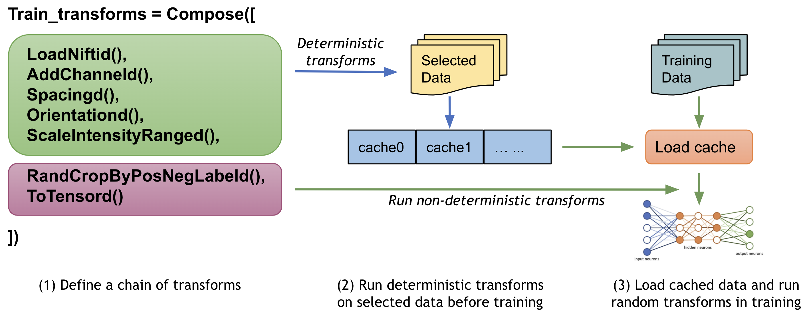
1. 訓練を高速化するためのキャッシュ IO と変換データ

ユーザは望まれるモデル品質を獲得するためにデータに渡り多くの (潜在的には数千の) エポックでモデルを訓練する必要が多くの場合あります。ネイティブ PyTorch 実装はデータを繰り返しロードして訓練の間総てのエポックについて同じ前処理ステップを実行する場合がありますが、これは時間がかかり不必要である可能性があります、特に医用画像ボリュームが大きいときには。

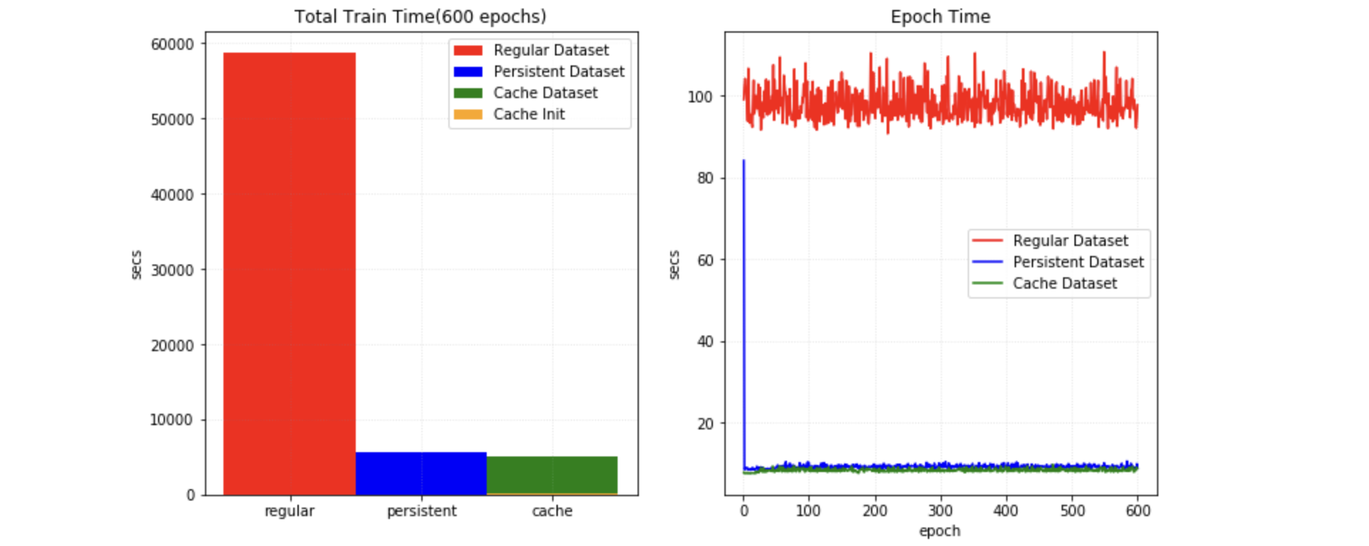
MONAI は、変換チェインの最初のランダム化された変換の前に、中間的な結果をストアして訓練の間これらの変換ステップを高速化するためにマルチスレッド CacheDataset と LMDBDataset を提供しています。この機能を有効にすると Datasets 実験の 10x 訓練スピードアップを潜在的に与えられるでしょう。

2. 中間結果を永続的なストレージにキャッシュする

PersistentDataset は CacheDataset に類似しています、そこでは (ハイパーパラメータ調整のときのような) 実験的な実行の間やデータセット全体のサイズが利用可能なメモリを越えるときの迅速な検索のために、中間的なキャッシュ値がディスク・ストレージや LMDB に永続化されます。PersistentDataset は Dataset 実験で CacheDataset と比較したとき同様の性能を獲得できました。

3. 大規模データベースのための SmartCache 機構

大規模なボリュームのデータセットによる訓練の間、効率的なアプローチはエポックでデータセットのサブセットだけを使用して訓練して総てのエポックでサブセットの部分を動的に置き換えることです。それは NVIDIA Clara-train SDK の SmartCache メカニズムです。

MONAI は PyTorch 版 SmartCache を SmartCacheDataset を提供しています。各エポックで、キャッシュの項目だけが訓練に使用され、同時に、別のスレッドがキャシュにない項目に変換シークエンスを提供することにより置換項目を準備しています。1 エポックが完了すれば、SmartCache は置換項目で同じ数の項目を置き換えます。

例えば、5 画像 : [image1, image2, image3, image4, image5] を持ち、そして cache_num=4, replace_rate=0.25 とします。するとキャッシュされて置換される、実際の訓練画像は以下のようになります :

epoch 1: [image1, image2, image3, image4]
epoch 2: [image2, image3, image4, image5]
epoch 3: [image3, image4, image5, image1]
epoch 3: [image4, image5, image1, image2]
epoch N: [image[N % 5] ...]

SmartCacheDataset の完全なサンプルは Distributed training with SmartCache で利用可能です。

4. マルチ PyTorch データセットの zip と出力の融合

MONAI は複数の PyTorch データセットを関連付けて出力データを (同じ対応するバッチインデックスで) タプルに連結するための ZipDataset を提供します、これは様々なデータソースに基づいて複雑な訓練プロセスを実行するの役立つことができます。

例えば :

class DatasetA(Dataset):
    def __getitem__(self, index: int):
        return image_data[index]

class DatasetB(Dataset):
    def __getitem__(self, index: int):
        return extra_data[index]

dataset = ZipDataset([DatasetA(), DatasetB()], transform)

5. PatchDataset

monai.data.PatchDataset は画像- とパッチ-レベル前処理の両方を組み合わせる柔軟な API を提供します :

image_dataset = Dataset(input_images, transforms=image_transforms)
patch_dataset = PatchDataset(
    dataset=image_dataset, patch_func=sampler,
    samples_per_image=n_samples, transform=patch_transforms)

それはカスタマイズ可能なパッチサンプリング・ストラテジーを使用してユーザ指定の image_transforms と patch_transforms をサポートします、これはマルチプロセス・コンテキストで 2 レベルの計算を切り離します。

6. 公開医療データの事前定義されたデータセット

医療ドメインのポピュラーな訓練データで素早く始めるために、MONAI は幾つかのデータ固有のデータセットを提供しています、これは AWS ストレージからのダウンロード、データファイルの抽出を含み、変換とともに訓練/評価項目の生成をサポートしています。そしてそれらはデフォルトの動作を変更する JSON config ファイルを簡単に変更できるという点で柔軟です。

MONAI は公開データセットの新しい寄与を常に歓迎しています、既存のデータセットを参照してダウンロードと抽出 API を活用してください、等々。公開データセット・チュートリアルは MedNISTDataset と DecathlonDataset で訓練ワークフローを素早くセットアップする方法と公開データのために新しいデータセットを作成する方法を示しています。

事前定義されたデータセットの一般的なワークフロー :

7. 交差検証のためにデータセットを分割する

MONAI の partition_dataset は訓練と検証のためあるいは交差検証のために様々なタイプの分割を実行できます。それは指定されたランダムシードに基づくシャッフルをサポートし、各データセットが一つの分割を含む、データセットのセットを返します。そしてそれは指定された比率に基づいてデータセットを分割したり、num_partitions に均等に分割することもできます。与えられたクラスラベルについて、総てのパーティションでクラスの同じ比率を確実にすることもできます。

8. CSV データセットと IterableDataset

CSV テーブルは画像データに加えて患者の人口統計, 検査結果, 画像収集パラメータと他の非画像データのような補助的な情報を組み込むためによく使用され、MONAI は CSV ファイルをロードするために CSVDataset をそしてスケーラブルなデータアクセスにより大規模な CSV ファイルをロードするために CSVIterableDataset をロードするために CSVIterableDataset を提供しています。ロードの間の通常の前処理変換に加えて、それはまた複数の CSV ファイルロード、テーブルの結合、行と列の選択とグループ化もサポートします。CSVDatasets チュートリアルは詳細な使用例を示しています。

9. ThreadDataLoader vs. DataLoader

変換が軽量である場合、特に総てのデータを RAM にキャッシュするとき、PyTorch DataLoader のマルチプロセッシングは不必要な IPC 時間を引き起こして総てのエポックの後に GPU 利用率の低下を引き起こす可能性があります。MONAI は変換を個別のスレッドで実行する ThreadDataLoader を提供しています :

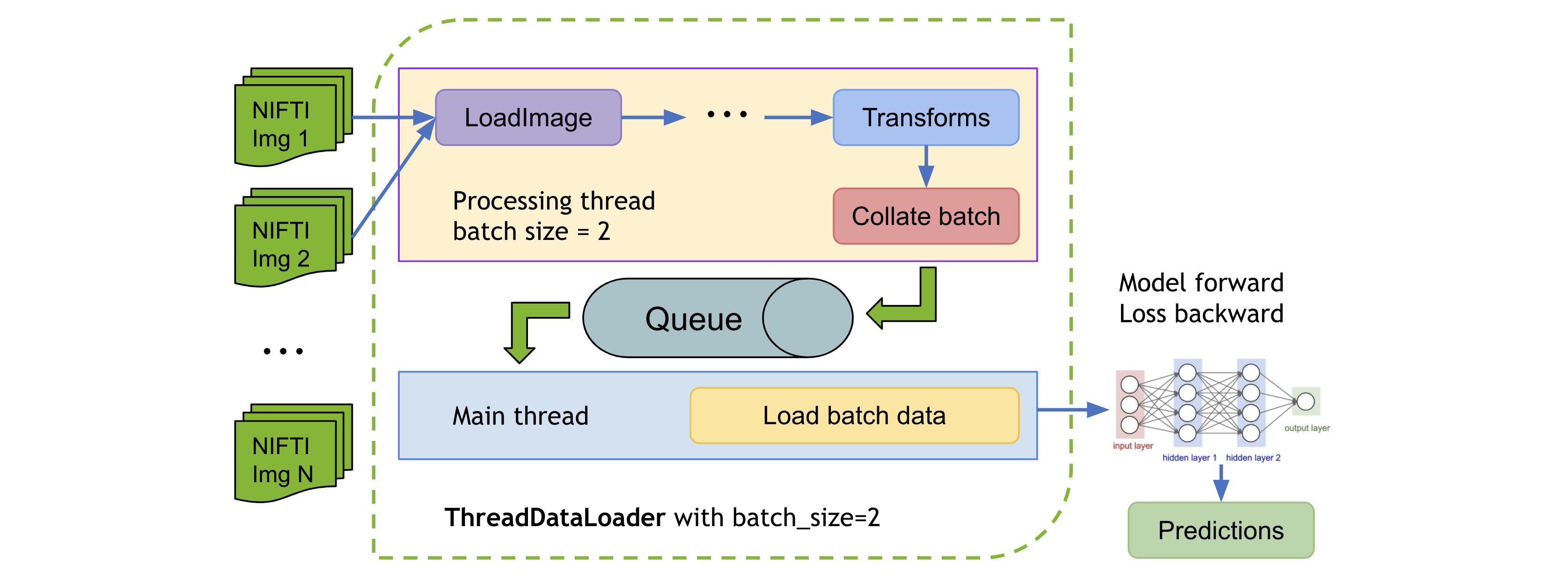
ThreadDataLoader サンプルは脾臓高速訓練チュートリアルで利用可能です。

以上

MONAI 0.7 : tutorials : モジュール – 脾臓セグメンテーション・タスクの後処理変換

10/17/2021

MONAI 0.7 : tutorials : モジュール – 脾臓セグメンテーション・タスクの後処理変換 (翻訳/解説)

翻訳 : (株)クラスキャットセールスインフォメーション
作成日時 : 10/17/2021 (0.7.0)

* 本ページは、MONAI の以下のドキュメントを翻訳した上で適宜、補足説明したものです：

Postprocessing Transforms with spleen segmentation task

クラスキャット人工知能研究開発支援サービス ★ 無料 Web セミナー開催中 ★

◆ クラスキャットは人工知能・テレワークに関する各種サービスを提供しております。お気軽にご相談ください :

人工知能研究開発支援
1. 人工知能研修サービス(経営者層向けオンサイト研修)
2. テクニカルコンサルティングサービス
3. 実証実験(プロトタイプ構築)
4. アプリケーションへの実装
人工知能研修サービス
PoC(概念実証)を失敗させないための支援
テレワーク & オンライン授業を支援

◆ 人工知能とビジネスをテーマに WEB セミナーを定期的に開催しています。スケジュール。

お住まいの地域に関係なく Web ブラウザからご参加頂けます。事前登録 が必要ですのでご注意ください。
ウェビナー運用には弊社製品「ClassCat® Webinar」を利用しています。

◆ お問合せ : 本件に関するお問い合わせ先は下記までお願いいたします。

株式会社クラスキャット セールス・マーケティング本部セールス・インフォメーション

E-Mail：sales-info@classcat.com ; WebSite: https://www.classcat.com/ ; Facebook

MONAI 0.7 : tutorials : モジュール – 脾臓セグメンテーション・タスクの後処理変換

このノートブックは脾臓セグメンテーション・タスクのモデル出力に基づいて幾つかの後処理変換の使用方法を示します。

MONAI はモデル出力を処理するための後処理変換を提供しています。現在、変換は以下を含みます :

Activations: 活性化層の追加 (Sigmoid, Softmax, etc.)。
AsDiscrete: 離散値 (Argmax, One-Hot, Threshold 値等) に変換します。
SplitChannel: マルチチャネル・データを複数のシングル・チャネルに分割する。
KeepLargestConnectedComponent: セグメンテーション結果の輪郭を抽出します、これは元の画像へのマップに使用できてモデルを評価できます。
LabelToContour: 接続コンポーネント分析に基づいてセグメンテーション・ノイズを除去する。

MONAI は同じデータ上で様々な前処理変換や後処理変換を適用して結果を結合するためのマルチ変換チェインをサポートしています、それはデータ辞書の指定された項目のコピーを作成する CopyItems 変換と想定される次元の指定項目を組み合わせるために ConcatItems 変換を提供し、そしてまたメモリを節約するために不要な項目を削除するための DeleteItems 変換も提供します。

典型的な使用方法は入力画像の 3 つの異なる強度範囲をスケールして結合することです :

このチュートリアルは脾臓セグメンテーションのモデル出力に基づいて上の後処理変換の幾つかを示します。

環境のセットアップ

!python -c "import monai" || pip install -q "monai-weekly[gdown, nibabel, skimage, tqdm]"
!python -c "import matplotlib" || pip install -q matplotlib
%matplotlib inline

from monai.utils import set_determinism
from monai.transforms import (
    AsDiscrete,
    AddChanneld,
    Compose,
    CropForegroundd,
    KeepLargestConnectedComponent,
    LabelToContour,
    LoadImaged,
    Orientationd,
    RandCropByPosNegLabeld,
    ScaleIntensityRanged,
    Spacingd,
    EnsureTyped,
    EnsureType,
)
from monai.networks.nets import UNet
from monai.networks.layers import Norm
from monai.metrics import DiceMetric
from monai.losses import DiceLoss
from monai.inferers import sliding_window_inference
from monai.data import CacheDataset, DataLoader, decollate_batch
from monai.config import print_config
from monai.apps import download_and_extract
import torch
import matplotlib.pyplot as plt
import tempfile
import shutil
import os
import glob

インポートのセットアップ

# Copyright 2020 MONAI Consortium
# Licensed under the Apache License, Version 2.0 (the "License");
# you may not use this file except in compliance with the License.
# You may obtain a copy of the License at
#     http://www.apache.org/licenses/LICENSE-2.0
# Unless required by applicable law or agreed to in writing, software
# distributed under the License is distributed on an "AS IS" BASIS,
# WITHOUT WARRANTIES OR CONDITIONS OF ANY KIND, either express or implied.
# See the License for the specific language governing permissions and
# limitations under the License.


print_config()

MONAI version: 0.6.0rc1+23.gc6793fd0
Numpy version: 1.20.3
Pytorch version: 1.9.0a0+c3d40fd
MONAI flags: HAS_EXT = True, USE_COMPILED = False
MONAI rev id: c6793fd0f316a448778d0047664aaf8c1895fe1c

Optional dependencies:
Pytorch Ignite version: 0.4.5
Nibabel version: 3.2.1
scikit-image version: 0.15.0
Pillow version: 7.0.0
Tensorboard version: 2.5.0
gdown version: 3.13.0
TorchVision version: 0.10.0a0
ITK version: 5.1.2
tqdm version: 4.53.0
lmdb version: 1.2.1
psutil version: 5.8.0
pandas version: 1.1.4
einops version: 0.3.0

For details about installing the optional dependencies, please visit:
    https://docs.monai.io/en/latest/installation.html#installing-the-recommended-dependencies

データディレクトリのセットアップ

directory = os.environ.get("MONAI_DATA_DIRECTORY")
root_dir = tempfile.mkdtemp() if directory is None else directory
print(root_dir)

/workspace/data/medical

データセットのダウンロード

データセットをダウンロードして展開します。データセットは http://medicaldecathlon.com/ に由来します。

resource = "https://msd-for-monai.s3-us-west-2.amazonaws.com/Task09_Spleen.tar"
md5 = "410d4a301da4e5b2f6f86ec3ddba524e"

compressed_file = os.path.join(root_dir, "Task09_Spleen.tar")
data_dir = os.path.join(root_dir, "Task09_Spleen")
if not os.path.exists(data_dir):
    download_and_extract(resource, compressed_file, root_dir, md5)

MSD 脾臓データセット・パスの設定

train_images = sorted(
    glob.glob(os.path.join(data_dir, "imagesTr", "*.nii.gz")))
train_labels = sorted(
    glob.glob(os.path.join(data_dir, "labelsTr", "*.nii.gz")))
data_dicts = [
    {"image": image_name, "label": label_name}
    for image_name, label_name in zip(train_images, train_labels)
]
train_files, val_files = data_dicts[:-9], data_dicts[-9:]

再現性のための決定論的訓練の設定

set_determinism(seed=0)

訓練と検証のための変換のセットアップ

train_transforms = Compose(
    [
        LoadImaged(keys=["image", "label"]),
        AddChanneld(keys=["image", "label"]),
        Spacingd(keys=["image", "label"], pixdim=(
            1.5, 1.5, 2.0), mode=("bilinear", "nearest")),
        Orientationd(keys=["image", "label"], axcodes="RAS"),
        ScaleIntensityRanged(
            keys=["image"], a_min=-57, a_max=164,
            b_min=0.0, b_max=1.0, clip=True,
        ),
        CropForegroundd(keys=["image", "label"], source_key="image"),
        # randomly crop out patch samples from big image
        # based on pos / neg ratio. the image centers
        # of negative samples must be in valid image area
        RandCropByPosNegLabeld(
            keys=["image", "label"],
            label_key="label",
            spatial_size=(96, 96, 96),
            pos=1,
            neg=1,
            num_samples=4,
            image_key="image",
            image_threshold=0,
        ),
        EnsureTyped(keys=["image", "label"]),
    ]
)
val_transforms = Compose(
    [
        LoadImaged(keys=["image", "label"]),
        AddChanneld(keys=["image", "label"]),
        Spacingd(keys=["image", "label"], pixdim=(
            1.5, 1.5, 2.0), mode=("bilinear", "nearest")),
        Orientationd(keys=["image", "label"], axcodes="RAS"),
        ScaleIntensityRanged(
            keys=["image"], a_min=-57, a_max=164,
            b_min=0.0, b_max=1.0, clip=True,
        ),
        CropForegroundd(keys=["image", "label"], source_key="image"),
        EnsureTyped(keys=["image", "label"]),
    ]
)

訓練と検証のための CacheDataset と DataLoader を定義する

train_ds = CacheDataset(
    data=train_files, transform=train_transforms,
    cache_rate=1.0, num_workers=4)
# train_ds = monai.data.Dataset(data=train_files, transform=train_transforms)

# use batch_size=2 to load images and use RandCropByPosNegLabeld
# to generate 2 x 4 images for network training
train_loader = DataLoader(train_ds, batch_size=2, shuffle=True, num_workers=4)

val_ds = CacheDataset(
    data=val_files, transform=val_transforms, cache_rate=1.0, num_workers=4)
# val_ds = monai.data.Dataset(data=val_files, transform=val_transforms)
val_loader = DataLoader(val_ds, batch_size=1, num_workers=4)

100%|██████████| 32/32 [00:48<00:00,  1.51s/it]
100%|██████████| 9/9 [00:11<00:00,  1.32s/it]

モデル、損失、Optimizer を作成する

# standard PyTorch program style: create UNet, DiceLoss and Adam optimizer
device = torch.device("cuda:0")
model = UNet(
    spatial_dims=3,
    in_channels=1,
    out_channels=2,
    channels=(16, 32, 64, 128, 256),
    strides=(2, 2, 2, 2),
    num_res_units=2,
    norm=Norm.BATCH,
).to(device)
loss_function = DiceLoss(to_onehot_y=True, softmax=True)
optimizer = torch.optim.Adam(model.parameters(), 1e-4)
dice_metric = DiceMetric(include_background=False, reduction="mean")

典型的な PyTorch 訓練プロセスを実行する

max_epochs = 160
val_interval = 2
best_metric = -1
best_metric_epoch = -1
epoch_loss_values = []
metric_values = []

post_pred = Compose([EnsureType(), AsDiscrete(argmax=True, to_onehot=True, num_classes=2)])
post_label = Compose([EnsureType(), AsDiscrete(to_onehot=True, num_classes=2)])

for epoch in range(max_epochs):
    print("-" * 10)
    print(f"epoch {epoch + 1}/{max_epochs}")
    model.train()
    epoch_loss = 0
    step = 0
    for batch_data in train_loader:
        step += 1
        inputs, labels = (
            batch_data["image"].to(device),
            batch_data["label"].to(device),
        )
        optimizer.zero_grad()
        outputs = model(inputs)
        loss = loss_function(outputs, labels)
        loss.backward()
        optimizer.step()
        epoch_loss += loss.item()
        print(
            f"{step}/{len(train_ds) // train_loader.batch_size},"
            f"train_loss: {loss.item():.4f}")
    epoch_loss /= step
    epoch_loss_values.append(epoch_loss)
    print(f"epoch {epoch + 1} average loss: {epoch_loss:.4f}")
    # validation progress
    if (epoch + 1) % val_interval == 0:
        model.eval()
        with torch.no_grad():
            for val_data in val_loader:
                val_inputs, val_labels = (
                    val_data["image"].to(device),
                    val_data["label"].to(device),
                )
                roi_size = (160, 160, 160)
                sw_batch_size = 4
                val_outputs = sliding_window_inference(
                    val_inputs, roi_size, sw_batch_size, model)
                val_outputs = [post_pred(i) for i in decollate_batch(val_outputs)]
                val_labels = [post_label(i) for i in decollate_batch(val_labels)]
                dice_metric(y_pred=val_outputs, y=val_labels)
            metric = dice_metric.aggregate().item()
            dice_metric.reset()
            metric_values.append(metric)
            if metric > best_metric:
                best_metric = metric
                best_metric_epoch = epoch + 1
                torch.save(model.state_dict(),
                           "best_metric_model_post_transforms.pth")
                print("saved new best metric model")
            print(
                f"current epoch: {epoch + 1} current mean dice: {metric:.4f}"
                f"\nbest mean dice: {best_metric:.4f} "
                f"at epoch: {best_metric_epoch}"
            )

検証データセット上で後処理変換を実行する

ここでは AsDiscrete, KeepLargestConnectedComponent と LabelToContour をテストします。

model.load_state_dict(torch.load("best_metric_model_post_transforms.pth"))
model.eval()
with torch.no_grad():
    for i, val_data in enumerate(val_loader):
        roi_size = (160, 160, 160)
        sw_batch_size = 4
        val_data = val_data["image"].to(device)
        val_output = sliding_window_inference(
            val_data, roi_size, sw_batch_size, model)
        # plot the slice [:, :, 80]
        plt.figure("check", (20, 4))
        plt.subplot(1, 5, 1)
        plt.title(f"image {i}")
        plt.imshow(val_data.detach().cpu()[0, 0, :, :, 80], cmap="gray")
        plt.subplot(1, 5, 2)
        plt.title(f"argmax {i}")
        argmax = [AsDiscrete(argmax=True)(i) for i in decollate_batch(val_output)]
        plt.imshow(argmax[0].detach().cpu()[0, :, :, 80])
        plt.subplot(1, 5, 3)
        plt.title(f"largest {i}")
        largest = [KeepLargestConnectedComponent(applied_labels=[1])(i) for i in argmax]
        plt.imshow(largest[0].detach().cpu()[0, :, :, 80])
        plt.subplot(1, 5, 4)
        plt.title(f"contour {i}")
        contour = [LabelToContour()(i) for i in largest]
        plt.imshow(contour[0].detach().cpu()[0, :, :, 80])
        plt.subplot(1, 5, 5)
        plt.title(f"map image {i}")
        map_image = contour[0] + val_data[0]
        plt.imshow(map_image.detach().cpu()[0, :, :, 80], cmap="gray")
        plt.show()

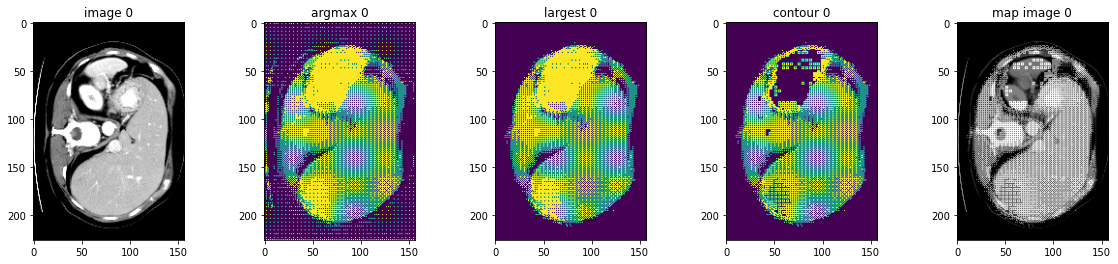
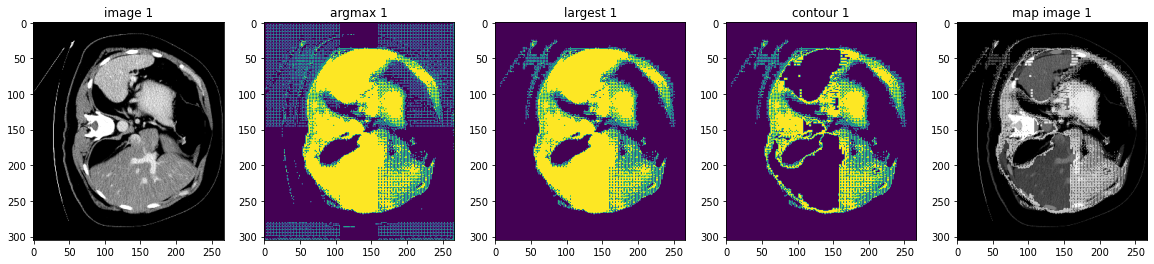
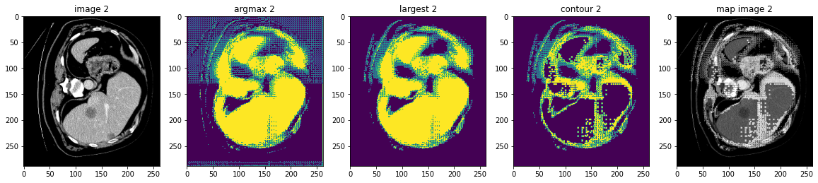
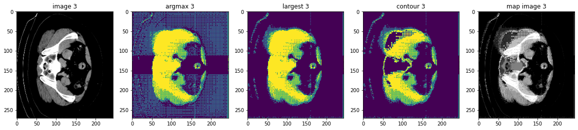
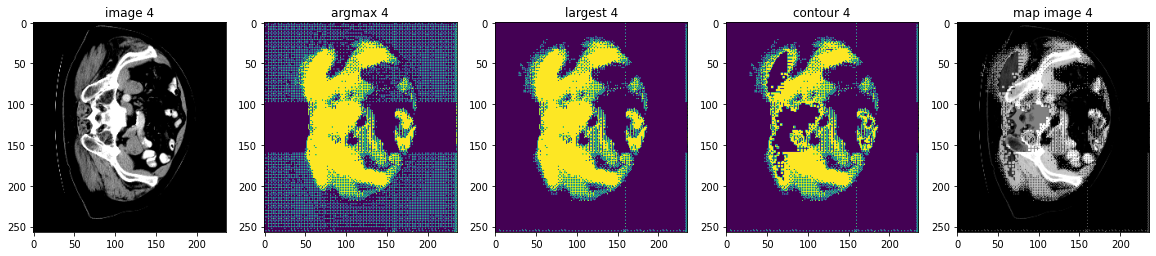
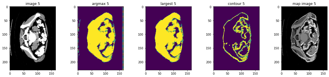
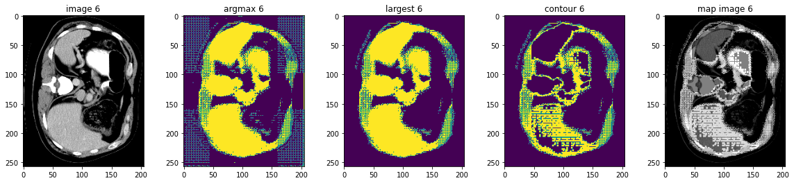
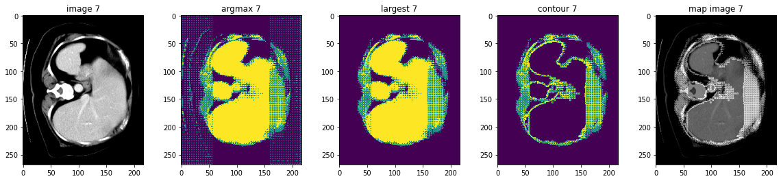
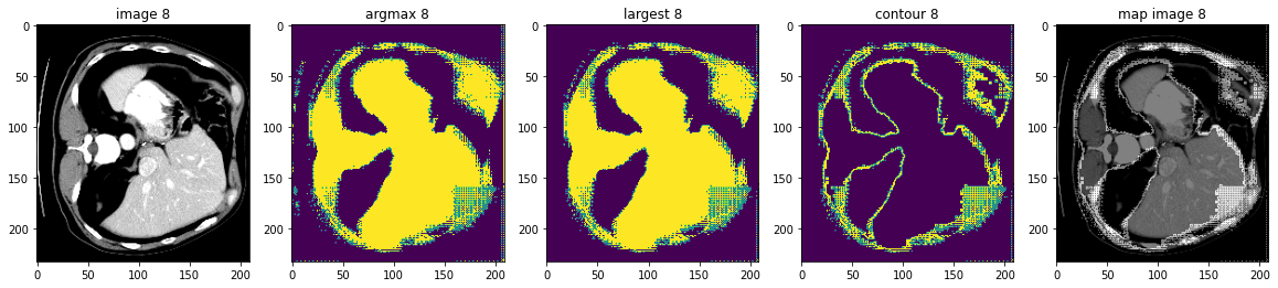
データディレクトリのクリーンアップ

一時ディレクトリが使用された場合にはディレクトリを削除します。

if directory is None:
    shutil.rmtree(root_dir)

以上

MONAI 0.7 : tutorials : 3D セグメンテーション – 脾臓 3D セグメンテーション (Lightning 版)

10/16/2021

MONAI 0.7 : tutorials : 3D セグメンテーション – 脾臓 3D セグメンテーション (Lightning 版) (翻訳/解説)

翻訳 : (株)クラスキャットセールスインフォメーション
作成日時 : 10/16/2021 (0.7.0)

* 本ページは、MONAI の以下のドキュメントを翻訳した上で適宜、補足説明したものです：

Spleen 3D segmentation with MONAI

クラスキャット人工知能研究開発支援サービス ★ 無料 Web セミナー開催中 ★

◆ クラスキャットは人工知能・テレワークに関する各種サービスを提供しております。お気軽にご相談ください :

人工知能研究開発支援
1. 人工知能研修サービス(経営者層向けオンサイト研修)
2. テクニカルコンサルティングサービス
3. 実証実験(プロトタイプ構築)
4. アプリケーションへの実装
人工知能研修サービス
PoC(概念実証)を失敗させないための支援
テレワーク & オンライン授業を支援

◆ 人工知能とビジネスをテーマに WEB セミナーを定期的に開催しています。スケジュール。

お住まいの地域に関係なく Web ブラウザからご参加頂けます。事前登録 が必要ですのでご注意ください。
ウェビナー運用には弊社製品「ClassCat® Webinar」を利用しています。

◆ お問合せ : 本件に関するお問い合わせ先は下記までお願いいたします。

株式会社クラスキャット セールス・マーケティング本部セールス・インフォメーション

E-Mail：sales-info@classcat.com ; WebSite: https://www.classcat.com/ ; Facebook

MONAI 0.7 : tutorials : 3D セグメンテーション – 脾臓 3D セグメンテーション (Lightning 版)

このノートブックは MONAI を PyTorch Lightning フレームワークと連携して使用できる可能性を示します。

このチュートリアルは MONAI をどのように PyTorch Lightning フレームワークと連携して使用できるかを実演します。

以下の MONAI の機能の使用方法を実演します :

辞書形式データのための変換。
メタデータとともに Nifti 画像をロードする。
チャネル次元がない場合チャネル dim をデータに追加する。
想定される範囲で医療画像強度をスケールする。
ポジティブ/ネガティブ・ラベル比率に基づいてバランスの取れた画像のバッチをクロップする。
訓練と検証を高速化するキャシュ IO と変換。
3D セグメンテーション・タスクのための 3D UNet モデル、Dice 損失関数、Mean Dice メトリック。
スライディング・ウィンドウ推論法。
再現性のための決定論的訓練。

Spleen データセットは http://medicaldecathlon.com/ からダウンロードできます。

Target: Spleen
Modality: CT
Size: 61 3D volumes (41 Training + 20 Testing)
Source: Memorial Sloan Kettering Cancer Center
Challenge: Large ranging foreground size

環境のセットアップ

!python -c "import monai" || pip install -q "monai-weekly[nibabel]"
!python -c "import matplotlib" || pip install -q matplotlib
!pip install -q pytorch-lightning==1.4.0
%matplotlib inline

WARNING: Running pip as the 'root' user can result in broken permissions and conflicting behaviour with the system package manager. It is recommended to use a virtual environment instead: https://pip.pypa.io/warnings/venv

インポートのセットアップ

# Copyright 2020 MONAI Consortium
# Licensed under the Apache License, Version 2.0 (the "License");
# you may not use this file except in compliance with the License.
# You may obtain a copy of the License at
#     http://www.apache.org/licenses/LICENSE-2.0
# Unless required by applicable law or agreed to in writing, software
# distributed under the License is distributed on an "AS IS" BASIS,
# WITHOUT WARRANTIES OR CONDITIONS OF ANY KIND, either express or implied.
# See the License for the specific language governing permissions and
# limitations under the License.

from monai.utils import set_determinism
from monai.transforms import (
    AsDiscrete,
    AddChanneld,
    Compose,
    CropForegroundd,
    LoadImaged,
    Orientationd,
    RandCropByPosNegLabeld,
    ScaleIntensityRanged,
    Spacingd,
    EnsureTyped,
    EnsureType,
)
from monai.networks.nets import UNet
from monai.networks.layers import Norm
from monai.metrics import DiceMetric
from monai.losses import DiceLoss
from monai.inferers import sliding_window_inference
from monai.data import CacheDataset, list_data_collate, decollate_batch
from monai.config import print_config
from monai.apps import download_and_extract
import torch
import pytorch_lightning
import matplotlib.pyplot as plt
import tempfile
import shutil
import os
import glob

print_config()

MONAI version: 0.6.0+1.g8365443a
Numpy version: 1.20.3
Pytorch version: 1.9.0a0+c3d40fd
MONAI flags: HAS_EXT = True, USE_COMPILED = False
MONAI rev id: 8365443ababac313340467e5987c7babe2b5b86a

Optional dependencies:
Pytorch Ignite version: 0.4.5
Nibabel version: 3.2.1
scikit-image version: 0.15.0
Pillow version: 8.2.0
Tensorboard version: 2.2.0
gdown version: 3.13.0
TorchVision version: 0.10.0a0
ITK version: 5.1.2
tqdm version: 4.53.0
lmdb version: 1.2.1
psutil version: 5.8.0
pandas version: 1.1.4
einops version: 0.3.0

For details about installing the optional dependencies, please visit:
    https://docs.monai.io/en/latest/installation.html#installing-the-recommended-dependencies

データディレクトリのセットアップ

directory = os.environ.get("MONAI_DATA_DIRECTORY")
root_dir = tempfile.mkdtemp() if directory is None else directory
print(root_dir)

/workspace/data/medical/

データセットのダウンロード

データセットをダウンロードして展開します。データセットは http://medicaldecathlon.com/ に由来します。

resource = "https://msd-for-monai.s3-us-west-2.amazonaws.com/Task09_Spleen.tar"
md5 = "410d4a301da4e5b2f6f86ec3ddba524e"

compressed_file = os.path.join(root_dir, "Task09_Spleen.tar")
data_dir = os.path.join(root_dir, "Task09_Spleen")
if not os.path.exists(data_dir):
    download_and_extract(resource, compressed_file, root_dir, md5)

LightningModule を定義する

LightningModule は訓練コードのリファクタリングを含みます。以下のモジュールは spleen_segmentation_3d.ipynb のコードのリファクタリングです :

class Net(pytorch_lightning.LightningModule):
    def __init__(self):
        super().__init__()
        self._model = UNet(
            spatial_dims=3,
            in_channels=1,
            out_channels=2,
            channels=(16, 32, 64, 128, 256),
            strides=(2, 2, 2, 2),
            num_res_units=2,
            norm=Norm.BATCH,
        )
        self.loss_function = DiceLoss(to_onehot_y=True, softmax=True)
        self.post_pred = Compose([EnsureType(), AsDiscrete(argmax=True, to_onehot=True, num_classes=2)])
        self.post_label = Compose([EnsureType(), AsDiscrete(to_onehot=True, num_classes=2)])
        self.dice_metric = DiceMetric(include_background=False, reduction="mean", get_not_nans=False)
        self.best_val_dice = 0
        self.best_val_epoch = 0

    def forward(self, x):
        return self._model(x)

    def prepare_data(self):
        # set up the correct data path
        train_images = sorted(
            glob.glob(os.path.join(data_dir, "imagesTr", "*.nii.gz")))
        train_labels = sorted(
            glob.glob(os.path.join(data_dir, "labelsTr", "*.nii.gz")))
        data_dicts = [
            {"image": image_name, "label": label_name}
            for image_name, label_name in zip(train_images, train_labels)
        ]
        train_files, val_files = data_dicts[:-9], data_dicts[-9:]

        # set deterministic training for reproducibility
        set_determinism(seed=0)

        # define the data transforms
        train_transforms = Compose(
            [
                LoadImaged(keys=["image", "label"]),
                AddChanneld(keys=["image", "label"]),
                Spacingd(
                    keys=["image", "label"],
                    pixdim=(1.5, 1.5, 2.0),
                    mode=("bilinear", "nearest"),
                ),
                Orientationd(keys=["image", "label"], axcodes="RAS"),
                ScaleIntensityRanged(
                    keys=["image"], a_min=-57, a_max=164,
                    b_min=0.0, b_max=1.0, clip=True,
                ),
                CropForegroundd(keys=["image", "label"], source_key="image"),
                # randomly crop out patch samples from
                # big image based on pos / neg ratio
                # the image centers of negative samples
                # must be in valid image area
                RandCropByPosNegLabeld(
                    keys=["image", "label"],
                    label_key="label",
                    spatial_size=(96, 96, 96),
                    pos=1,
                    neg=1,
                    num_samples=4,
                    image_key="image",
                    image_threshold=0,
                ),
                # user can also add other random transforms
                #                 RandAffined(
                #                     keys=['image', 'label'],
                #                     mode=('bilinear', 'nearest'),
                #                     prob=1.0,
                #                     spatial_size=(96, 96, 96),
                #                     rotate_range=(0, 0, np.pi/15),
                #                     scale_range=(0.1, 0.1, 0.1)),
                EnsureTyped(keys=["image", "label"]),
            ]
        )
        val_transforms = Compose(
            [
                LoadImaged(keys=["image", "label"]),
                AddChanneld(keys=["image", "label"]),
                Spacingd(
                    keys=["image", "label"],
                    pixdim=(1.5, 1.5, 2.0),
                    mode=("bilinear", "nearest"),
                ),
                Orientationd(keys=["image", "label"], axcodes="RAS"),
                ScaleIntensityRanged(
                    keys=["image"], a_min=-57, a_max=164,
                    b_min=0.0, b_max=1.0, clip=True,
                ),
                CropForegroundd(keys=["image", "label"], source_key="image"),
                EnsureTyped(keys=["image", "label"]),
            ]
        )

        # we use cached datasets - these are 10x faster than regular datasets
        self.train_ds = CacheDataset(
            data=train_files, transform=train_transforms,
            cache_rate=1.0, num_workers=4,
        )
        self.val_ds = CacheDataset(
            data=val_files, transform=val_transforms,
            cache_rate=1.0, num_workers=4,
        )
#         self.train_ds = monai.data.Dataset(
#             data=train_files, transform=train_transforms)
#         self.val_ds = monai.data.Dataset(
#             data=val_files, transform=val_transforms)

    def train_dataloader(self):
        train_loader = torch.utils.data.DataLoader(
            self.train_ds, batch_size=2, shuffle=True,
            num_workers=4, collate_fn=list_data_collate,
        )
        return train_loader

    def val_dataloader(self):
        val_loader = torch.utils.data.DataLoader(
            self.val_ds, batch_size=1, num_workers=4)
        return val_loader

    def configure_optimizers(self):
        optimizer = torch.optim.Adam(self._model.parameters(), 1e-4)
        return optimizer

    def training_step(self, batch, batch_idx):
        images, labels = batch["image"], batch["label"]
        output = self.forward(images)
        loss = self.loss_function(output, labels)
        tensorboard_logs = {"train_loss": loss.item()}
        return {"loss": loss, "log": tensorboard_logs}

    def validation_step(self, batch, batch_idx):
        images, labels = batch["image"], batch["label"]
        roi_size = (160, 160, 160)
        sw_batch_size = 4
        outputs = sliding_window_inference(
            images, roi_size, sw_batch_size, self.forward)
        loss = self.loss_function(outputs, labels)
        outputs = [self.post_pred(i) for i in decollate_batch(outputs)]
        labels = [self.post_label(i) for i in decollate_batch(labels)]
        self.dice_metric(y_pred=outputs, y=labels)
        return {"val_loss": loss, "val_number": len(outputs)}

    def validation_epoch_end(self, outputs):
        val_loss, num_items = 0, 0
        for output in outputs:
            val_loss += output["val_loss"].sum().item()
            num_items += output["val_number"]
        mean_val_dice = self.dice_metric.aggregate().item()
        self.dice_metric.reset()
        mean_val_loss = torch.tensor(val_loss / num_items)
        tensorboard_logs = {
            "val_dice": mean_val_dice,
            "val_loss": mean_val_loss,
        }
        if mean_val_dice > self.best_val_dice:
            self.best_val_dice = mean_val_dice
            self.best_val_epoch = self.current_epoch
        print(
            f"current epoch: {self.current_epoch} "
            f"current mean dice: {mean_val_dice:.4f}"
            f"\nbest mean dice: {self.best_val_dice:.4f} "
            f"at epoch: {self.best_val_epoch}"
        )
        return {"log": tensorboard_logs}

訓練の実行

# initialise the LightningModule
net = Net()

# set up loggers and checkpoints
log_dir = os.path.join(root_dir, "logs")
tb_logger = pytorch_lightning.loggers.TensorBoardLogger(
    save_dir=log_dir
)

# initialise Lightning's trainer.
trainer = pytorch_lightning.Trainer(
    gpus=[0],
    max_epochs=600,
    logger=tb_logger,
    checkpoint_callback=True,
    num_sanity_val_steps=1,
)

# train
trainer.fit(net)

print(
    f"train completed, best_metric: {net.best_val_dice:.4f} "
    f"at epoch {net.best_val_epoch}")

train completed, best_metric: 0.9498 at epoch 563

tensorboard で訓練を見る

%load_ext tensorboard
%tensorboard --logdir=log_dir

The tensorboard extension is already loaded. To reload it, use:
  %reload_ext tensorboard
Reusing TensorBoard on port 6006 (pid 27668), started 1:35:41 ago. (Use '!kill 27668' to kill it.)

入力画像とラベルでベストなモデル出力を確認する

net.eval()
device = torch.device("cuda:0")
net.to(device)
with torch.no_grad():
    for i, val_data in enumerate(net.val_dataloader()):
        roi_size = (160, 160, 160)
        sw_batch_size = 4
        val_outputs = sliding_window_inference(
            val_data["image"].to(device), roi_size, sw_batch_size, net
        )
        # plot the slice [:, :, 80]
        plt.figure("check", (18, 6))
        plt.subplot(1, 3, 1)
        plt.title(f"image {i}")
        plt.imshow(val_data["image"][0, 0, :, :, 80], cmap="gray")
        plt.subplot(1, 3, 2)
        plt.title(f"label {i}")
        plt.imshow(val_data["label"][0, 0, :, :, 80])
        plt.subplot(1, 3, 3)
        plt.title(f"output {i}")
        plt.imshow(torch.argmax(
            val_outputs, dim=1).detach().cpu()[0, :, :, 80])
        plt.show()

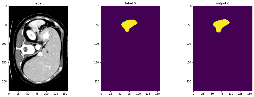
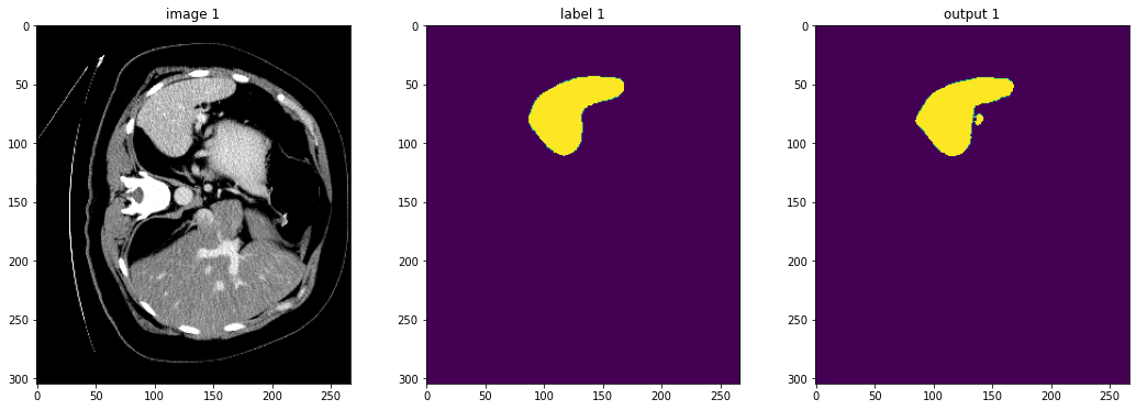
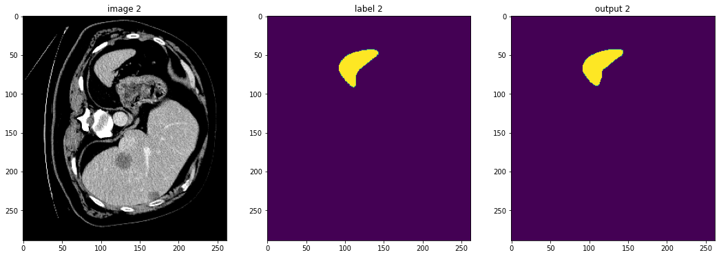
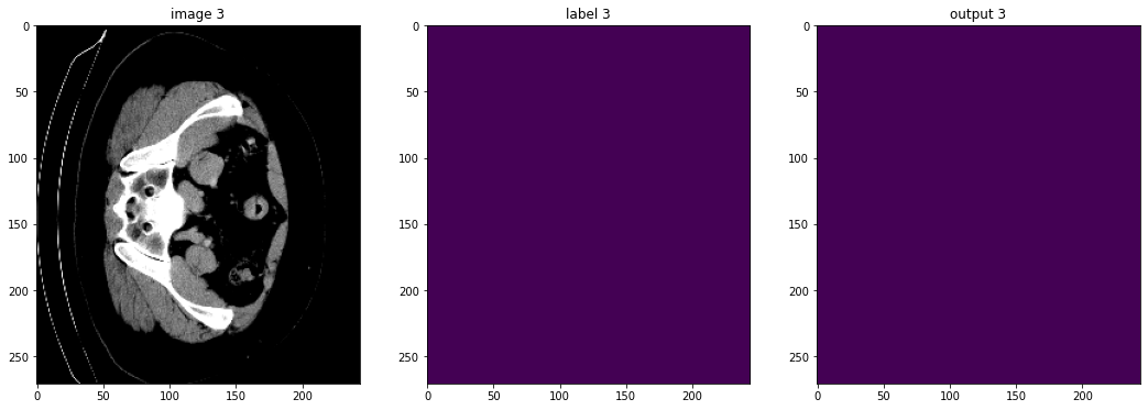
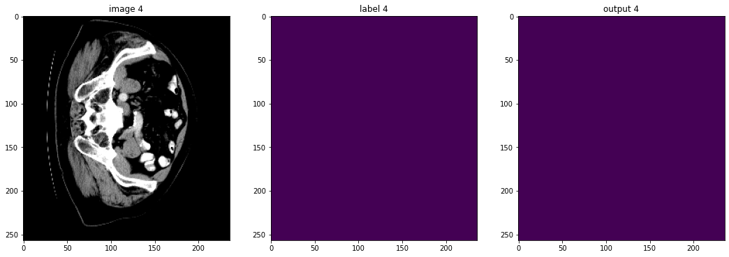
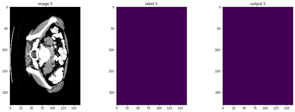
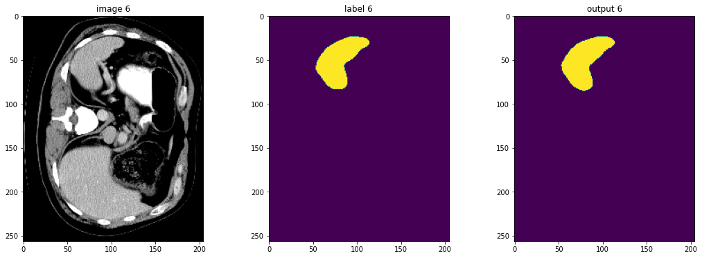
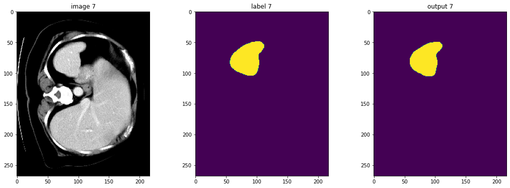
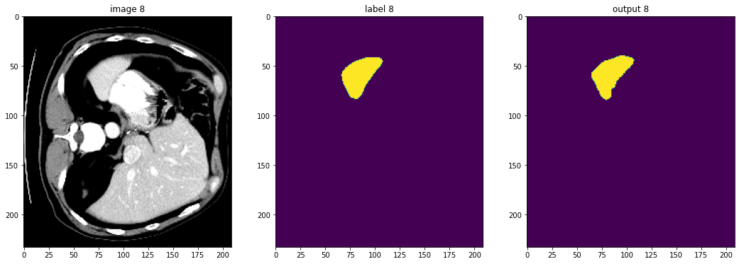
データディレクトリのクリーンアップ

一時ディレクトリが使用された場合はディレクトリを削除する。

if directory is None:
    shutil.rmtree(root_dir)

以上

MONAI 0.7 : tutorials : 3D セグメンテーション – 脾臓 3D セグメンテーション

10/16/2021

MONAI 0.7 : tutorials : 3D セグメンテーション – 脾臓 3D セグメンテーション (翻訳/解説)

翻訳 : (株)クラスキャットセールスインフォメーション
作成日時 : 10/16/2021 (0.7.0)

* 本ページは、MONAI の以下のドキュメントを翻訳した上で適宜、補足説明したものです：

Spleen 3D segmentation with MONAI

クラスキャット人工知能研究開発支援サービス ★ 無料 Web セミナー開催中 ★

◆ クラスキャットは人工知能・テレワークに関する各種サービスを提供しております。お気軽にご相談ください :

人工知能研究開発支援
1. 人工知能研修サービス(経営者層向けオンサイト研修)
2. テクニカルコンサルティングサービス
3. 実証実験(プロトタイプ構築)
4. アプリケーションへの実装
人工知能研修サービス
PoC(概念実証)を失敗させないための支援
テレワーク & オンライン授業を支援

◆ 人工知能とビジネスをテーマに WEB セミナーを定期的に開催しています。スケジュール。

お住まいの地域に関係なく Web ブラウザからご参加頂けます。事前登録 が必要ですのでご注意ください。
ウェビナー運用には弊社製品「ClassCat® Webinar」を利用しています。

◆ お問合せ : 本件に関するお問い合わせ先は下記までお願いいたします。

株式会社クラスキャット セールス・マーケティング本部セールス・インフォメーション

E-Mail：sales-info@classcat.com ; WebSite: https://www.classcat.com/ ; Facebook

MONAI 0.7 : tutorials : 3D セグメンテーション – 脾臓 3D セグメンテーション

このノートブックは MSD 脾臓データセットに基づいた 3D セグメンテーションの end-to-end な訓練と評価サンプルです。このサンプルは PyTorch ベースのプログラムで MONAI モジュールの柔軟性を示します :

辞書ベースの訓練データ構造のための変換。
メタデータと共に NIfTI 画像をロードする。
想定する範囲で医療画像強度をスケールする。
ポジティブ/ネガティブ・ラベル比率に基づいてバランスの取れた画像パッチサンプルのバッチをクロップする。
訓練と検証を高速化するキャッシュ IO と変換。
3D セグメンテーション・タスクのための 3D UNet, Dice 損失関数, Mean Dice メトリック。
スライディング・ウィンドウ推論。
再現性のための決定論的訓練。

このチュートリアルは MONAI を既存の PyTorch 医療 DL プログラムに統合する方法を示します。

そして以下の機能を簡単に使用することができます :

辞書形式データのための変換。
メタデータとともに Nifti 画像をロードする。
チャネル次元がない場合チャネル dim をデータに追加する。
想定される範囲で医療画像強度をスケールする。
ポジティブ/ネガティブ・ラベル比率に基づいてバランスの取れた画像のバッチをクロップする。
訓練と検証を高速化するキャシュ IO と変換。
3D セグメンテーション・タスクのための 3D UNet モデル、Dice 損失関数、Mean Dice メトリック。
スライディング・ウィンドウ推論法。
再現性のための決定論的訓練。

Spleen データセットは http://medicaldecathlon.com/ からダウンロードできます。

Target: Spleen
Modality: CT
Size: 61 3D volumes (41 Training + 20 Testing)
Source: Memorial Sloan Kettering Cancer Center
Challenge: Large ranging foreground size

環境のセットアップ

!python -c "import monai" || pip install -q "monai-weekly[gdown, nibabel, tqdm]"
!python -c "import matplotlib" || pip install -q matplotlib
%matplotlib inline

from monai.utils import first, set_determinism
from monai.transforms import (
    AsDiscrete,
    AsDiscreted,
    EnsureChannelFirstd,
    Compose,
    CropForegroundd,
    LoadImaged,
    Orientationd,
    RandCropByPosNegLabeld,
    ScaleIntensityRanged,
    Spacingd,
    EnsureTyped,
    EnsureType,
    Invertd,
)
from monai.handlers.utils import from_engine
from monai.networks.nets import UNet
from monai.networks.layers import Norm
from monai.metrics import DiceMetric
from monai.losses import DiceLoss
from monai.inferers import sliding_window_inference
from monai.data import CacheDataset, DataLoader, Dataset, decollate_batch
from monai.config import print_config
from monai.apps import download_and_extract
import torch
import matplotlib.pyplot as plt
import tempfile
import shutil
import os
import glob

インポートのセットアップ

# Copyright 2020 MONAI Consortium
# Licensed under the Apache License, Version 2.0 (the "License");
# you may not use this file except in compliance with the License.
# You may obtain a copy of the License at
#     http://www.apache.org/licenses/LICENSE-2.0
# Unless required by applicable law or agreed to in writing, software
# distributed under the License is distributed on an "AS IS" BASIS,
# WITHOUT WARRANTIES OR CONDITIONS OF ANY KIND, either express or implied.
# See the License for the specific language governing permissions and
# limitations under the License.


print_config()

MONAI version: 0.6.0+22.g027947bf
Numpy version: 1.20.3
Pytorch version: 1.9.0a0+c3d40fd
MONAI flags: HAS_EXT = False, USE_COMPILED = False
MONAI rev id: 027947bf91ff0dfac94f472ed1855cd49e3feb8d

Optional dependencies:
Pytorch Ignite version: 0.4.5
Nibabel version: 3.2.1
scikit-image version: 0.15.0
Pillow version: 8.2.0
Tensorboard version: 2.5.0
gdown version: 3.13.0
TorchVision version: 0.10.0a0
tqdm version: 4.53.0
lmdb version: 1.2.1
psutil version: 5.8.0
pandas version: 1.1.4
einops version: 0.3.0

For details about installing the optional dependencies, please visit:
    https://docs.monai.io/en/latest/installation.html#installing-the-recommended-dependencies

データディレクトリのセットアップ

directory = os.environ.get("MONAI_DATA_DIRECTORY")
root_dir = tempfile.mkdtemp() if directory is None else directory
print(root_dir)

/workspace/data/medical/

データセットのダウンロード

データセットをダウンロードして展開します。データセットは http://medicaldecathlon.com/ に由来します。

resource = "https://msd-for-monai.s3-us-west-2.amazonaws.com/Task09_Spleen.tar"
md5 = "410d4a301da4e5b2f6f86ec3ddba524e"

compressed_file = os.path.join(root_dir, "Task09_Spleen.tar")
data_dir = os.path.join(root_dir, "Task09_Spleen")
if not os.path.exists(data_dir):
    download_and_extract(resource, compressed_file, root_dir, md5)

MSD 脾臓データセット・パスの設定

train_images = sorted(
    glob.glob(os.path.join(data_dir, "imagesTr", "*.nii.gz")))
train_labels = sorted(
    glob.glob(os.path.join(data_dir, "labelsTr", "*.nii.gz")))
data_dicts = [
    {"image": image_name, "label": label_name}
    for image_name, label_name in zip(train_images, train_labels)
]
train_files, val_files = data_dicts[:-9], data_dicts[-9:]

再現性のための決定論的訓練の設定

set_determinism(seed=0)

訓練と検証のための変換のセットアップ

ここではデータセットを増強するために幾つかの変換を使用します :

LoadImaged は NIfTI 形式ファイルから脾臓 CT 画像とラベルをロードします。
AddChanneld は元のデータがチャネル dim を持たないとき、「チャネル first」shape を構築するために 1 dim 追加します。
Spacingd はアフィン行列に基づいて pixdim=(1.5, 1.5, 2.) により spacing を調整します。
Orientationd はアフィン行列に基づいてデータの向きを統一します。
ScaleIntensityRanged は強度範囲 [-57, 164] を抽出して [0, 1] にスケールします。
CropForegroundd は画像とラベルの valid body 領域にフォーカスするために総てのゼロ境界 (= border) を削除します。
RandCropByPosNegLabeld は pos / neg 比率に基づいて大きな画像からランダムにパッチサンプルをクロップします。
ネガティブサンプルの画像の中心は valid body 領域内になければなりません。
RandAffined は PyTorch アフィン変換に基づいて回転, スケール, shear, 並行移動等を一緒に効率的に実行します。
EnsureTyped は更なるステップのために numpy 配列を PyTorch テンソルに変換します。

train_transforms = Compose(
    [
        LoadImaged(keys=["image", "label"]),
        EnsureChannelFirstd(keys=["image", "label"]),
        Spacingd(keys=["image", "label"], pixdim=(
            1.5, 1.5, 2.0), mode=("bilinear", "nearest")),
        Orientationd(keys=["image", "label"], axcodes="RAS"),
        ScaleIntensityRanged(
            keys=["image"], a_min=-57, a_max=164,
            b_min=0.0, b_max=1.0, clip=True,
        ),
        CropForegroundd(keys=["image", "label"], source_key="image"),
        RandCropByPosNegLabeld(
            keys=["image", "label"],
            label_key="label",
            spatial_size=(96, 96, 96),
            pos=1,
            neg=1,
            num_samples=4,
            image_key="image",
            image_threshold=0,
        ),
        # user can also add other random transforms
        # RandAffined(
        #     keys=['image', 'label'],
        #     mode=('bilinear', 'nearest'),
        #     prob=1.0, spatial_size=(96, 96, 96),
        #     rotate_range=(0, 0, np.pi/15),
        #     scale_range=(0.1, 0.1, 0.1)),
        EnsureTyped(keys=["image", "label"]),
    ]
)
val_transforms = Compose(
    [
        LoadImaged(keys=["image", "label"]),
        EnsureChannelFirstd(keys=["image", "label"]),
        Spacingd(keys=["image", "label"], pixdim=(
            1.5, 1.5, 2.0), mode=("bilinear", "nearest")),
        Orientationd(keys=["image", "label"], axcodes="RAS"),
        ScaleIntensityRanged(
            keys=["image"], a_min=-57, a_max=164,
            b_min=0.0, b_max=1.0, clip=True,
        ),
        CropForegroundd(keys=["image", "label"], source_key="image"),
        EnsureTyped(keys=["image", "label"]),
    ]
)

DataLoaer で変換を確認する

check_ds = Dataset(data=val_files, transform=val_transforms)
check_loader = DataLoader(check_ds, batch_size=1)
check_data = first(check_loader)
image, label = (check_data["image"][0][0], check_data["label"][0][0])
print(f"image shape: {image.shape}, label shape: {label.shape}")
# plot the slice [:, :, 80]
plt.figure("check", (12, 6))
plt.subplot(1, 2, 1)
plt.title("image")
plt.imshow(image[:, :, 80], cmap="gray")
plt.subplot(1, 2, 2)
plt.title("label")
plt.imshow(label[:, :, 80])
plt.show()

image shape: torch.Size([226, 157, 113]), label shape: torch.Size([226, 157, 113])

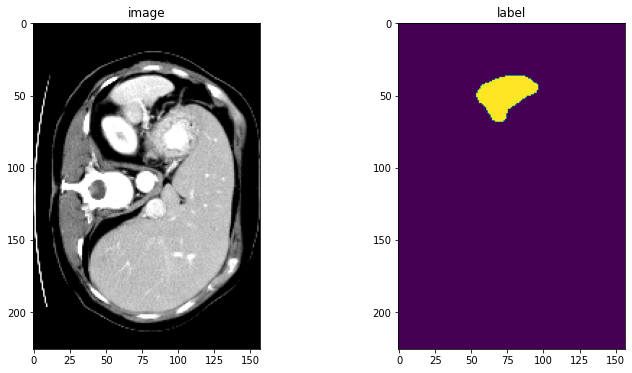
訓練と検証のために CacheDataset と DataLoader を定義する

ここで訓練と検証プロセスを高速化するために CacheDataset を使用し、それは通常の Dataset よりも 10x 高速です。ベストなパフォーマンスを得るためには、総てのデータをキャッシュするために cache_rate=1.0 を設定します、メモリが十分でない場合には、低い値を設定してください。ユーザはまた cache_rate の代わりに cache_num を設定することもできて、2 つの設定の最小値を使用します。そしてキャッシュの間にマルチスレッドを有効にするために num_workers を設定します。通常の Dataset を試したい場合は、下でコメントされたコードを単に使用するように変更してください。

train_ds = CacheDataset(
    data=train_files, transform=train_transforms,
    cache_rate=1.0, num_workers=4)
# train_ds = monai.data.Dataset(data=train_files, transform=train_transforms)

# use batch_size=2 to load images and use RandCropByPosNegLabeld
# to generate 2 x 4 images for network training
train_loader = DataLoader(train_ds, batch_size=2, shuffle=True, num_workers=4)

val_ds = CacheDataset(
    data=val_files, transform=val_transforms, cache_rate=1.0, num_workers=4)
# val_ds = Dataset(data=val_files, transform=val_transforms)
val_loader = DataLoader(val_ds, batch_size=1, num_workers=4)

Loading dataset: 100%|██████████| 32/32 [00:32<00:00,  1.02s/it]
Loading dataset: 100%|██████████| 9/9 [00:07<00:00,  1.18it/s]

モデル、損失、Optimizer を作成する

# standard PyTorch program style: create UNet, DiceLoss and Adam optimizer
device = torch.device("cuda:0")
model = UNet(
    spatial_dims=3,
    in_channels=1,
    out_channels=2,
    channels=(16, 32, 64, 128, 256),
    strides=(2, 2, 2, 2),
    num_res_units=2,
    norm=Norm.BATCH,
).to(device)
loss_function = DiceLoss(to_onehot_y=True, softmax=True)
optimizer = torch.optim.Adam(model.parameters(), 1e-4)
dice_metric = DiceMetric(include_background=False, reduction="mean")

典型的な PyTorch 訓練プロセスを実行する

max_epochs = 600
val_interval = 2
best_metric = -1
best_metric_epoch = -1
epoch_loss_values = []
metric_values = []
post_pred = Compose([EnsureType(), AsDiscrete(argmax=True, to_onehot=True, num_classes=2)])
post_label = Compose([EnsureType(), AsDiscrete(to_onehot=True, num_classes=2)])

for epoch in range(max_epochs):
    print("-" * 10)
    print(f"epoch {epoch + 1}/{max_epochs}")
    model.train()
    epoch_loss = 0
    step = 0
    for batch_data in train_loader:
        step += 1
        inputs, labels = (
            batch_data["image"].to(device),
            batch_data["label"].to(device),
        )
        optimizer.zero_grad()
        outputs = model(inputs)
        loss = loss_function(outputs, labels)
        loss.backward()
        optimizer.step()
        epoch_loss += loss.item()
        print(
            f"{step}/{len(train_ds) // train_loader.batch_size}, "
            f"train_loss: {loss.item():.4f}")
    epoch_loss /= step
    epoch_loss_values.append(epoch_loss)
    print(f"epoch {epoch + 1} average loss: {epoch_loss:.4f}")

    if (epoch + 1) % val_interval == 0:
        model.eval()
        with torch.no_grad():
            for val_data in val_loader:
                val_inputs, val_labels = (
                    val_data["image"].to(device),
                    val_data["label"].to(device),
                )
                roi_size = (160, 160, 160)
                sw_batch_size = 4
                val_outputs = sliding_window_inference(
                    val_inputs, roi_size, sw_batch_size, model)
                val_outputs = [post_pred(i) for i in decollate_batch(val_outputs)]
                val_labels = [post_label(i) for i in decollate_batch(val_labels)]
                # compute metric for current iteration
                dice_metric(y_pred=val_outputs, y=val_labels)

            # aggregate the final mean dice result
            metric = dice_metric.aggregate().item()
            # reset the status for next validation round
            dice_metric.reset()

            metric_values.append(metric)
            if metric > best_metric:
                best_metric = metric
                best_metric_epoch = epoch + 1
                torch.save(model.state_dict(), os.path.join(
                    root_dir, "best_metric_model.pth"))
                print("saved new best metric model")
            print(
                f"current epoch: {epoch + 1} current mean dice: {metric:.4f}"
                f"\nbest mean dice: {best_metric:.4f} "
                f"at epoch: {best_metric_epoch}"
            )

print(
    f"train completed, best_metric: {best_metric:.4f} "
    f"at epoch: {best_metric_epoch}")

train completed, best_metric: 0.9510 at epoch: 598

損失とメトリックをプロットする


plt.figure("train", (12, 6))
plt.subplot(1, 2, 1)
plt.title("Epoch Average Loss")
x = [i + 1 for i in range(len(epoch_loss_values))]
y = epoch_loss_values
plt.xlabel("epoch")
plt.plot(x, y)
plt.subplot(1, 2, 2)
plt.title("Val Mean Dice")
x = [val_interval * (i + 1) for i in range(len(metric_values))]
y = metric_values
plt.xlabel("epoch")
plt.plot(x, y)
plt.show()

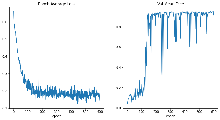
入力画像とラベルでベストなモデル出力を確認する

model.load_state_dict(torch.load(
    os.path.join(root_dir, "best_metric_model.pth")))
model.eval()
with torch.no_grad():
    for i, val_data in enumerate(val_loader):
        roi_size = (160, 160, 160)
        sw_batch_size = 4
        val_outputs = sliding_window_inference(
            val_data["image"].to(device), roi_size, sw_batch_size, model
        )
        # plot the slice [:, :, 80]
        plt.figure("check", (18, 6))
        plt.subplot(1, 3, 1)
        plt.title(f"image {i}")
        plt.imshow(val_data["image"][0, 0, :, :, 80], cmap="gray")
        plt.subplot(1, 3, 2)
        plt.title(f"label {i}")
        plt.imshow(val_data["label"][0, 0, :, :, 80])
        plt.subplot(1, 3, 3)
        plt.title(f"output {i}")
        plt.imshow(torch.argmax(
            val_outputs, dim=1).detach().cpu()[0, :, :, 80])
        plt.show()
        if i == 2:
            break

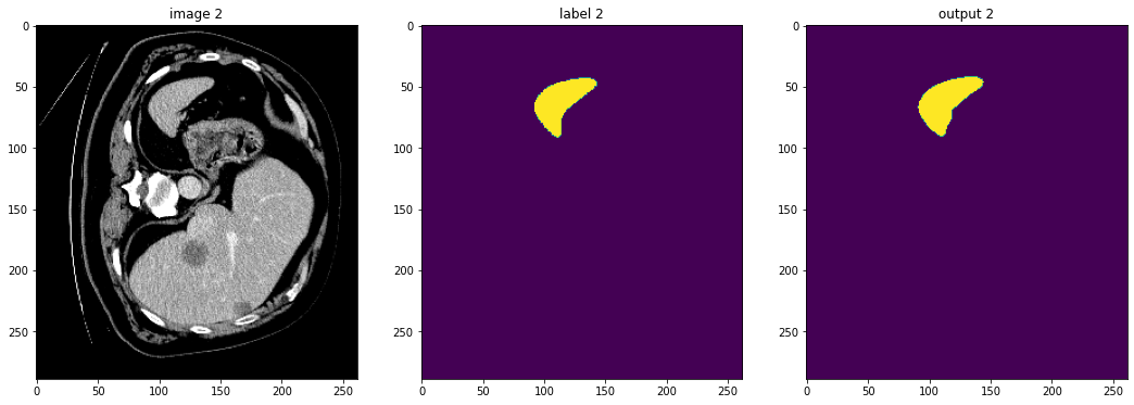
元の画像 spacing 上の評価

val_org_transforms = Compose(
    [
        LoadImaged(keys=["image", "label"]),
        EnsureChannelFirstd(keys=["image", "label"]),
        Spacingd(keys=["image"], pixdim=(
            1.5, 1.5, 2.0), mode="bilinear"),
        Orientationd(keys=["image"], axcodes="RAS"),
        ScaleIntensityRanged(
            keys=["image"], a_min=-57, a_max=164,
            b_min=0.0, b_max=1.0, clip=True,
        ),
        CropForegroundd(keys=["image"], source_key="image"),
        EnsureTyped(keys=["image", "label"]),
    ]
)

val_org_ds = Dataset(
    data=val_files, transform=val_org_transforms)
val_org_loader = DataLoader(val_org_ds, batch_size=1, num_workers=4)

post_transforms = Compose([
    EnsureTyped(keys="pred"),
    Invertd(
        keys="pred",
        transform=val_org_transforms,
        orig_keys="image",
        meta_keys="pred_meta_dict",
        orig_meta_keys="image_meta_dict",
        meta_key_postfix="meta_dict",
        nearest_interp=False,
        to_tensor=True,
    ),
    AsDiscreted(keys="pred", argmax=True, to_onehot=True, num_classes=2),
    AsDiscreted(keys="label", to_onehot=True, num_classes=2),
])

model.load_state_dict(torch.load(
    os.path.join(root_dir, "best_metric_model.pth")))
model.eval()

with torch.no_grad():
    for val_data in val_org_loader:
        val_inputs = val_data["image"].to(device)
        roi_size = (160, 160, 160)
        sw_batch_size = 4
        val_data["pred"] = sliding_window_inference(
            val_inputs, roi_size, sw_batch_size, model)
        val_data = [post_transforms(i) for i in decollate_batch(val_data)]
        val_outputs, val_labels = from_engine(["pred", "label"])(val_data)
        # compute metric for current iteration
        dice_metric(y_pred=val_outputs, y=val_labels)

    # aggregate the final mean dice result
    metric_org = dice_metric.aggregate().item()
    # reset the status for next validation round
    dice_metric.reset()

print("Metric on original image spacing: ", metric_org)

Metric on original image spacing:  0.9637420177459717

データディレクトリのクリーンアップ

一時ディレクトリが使用された場合にはディレクトリを削除します。

if directory is None:
    shutil.rmtree(root_dir)

以上