MONAI 1.0 : tutorials : 3D セグメンテーション – 脳腫瘍 3D セグメンテーション (翻訳/解説)

翻訳 : (株)クラスキャット セールスインフォメーション
作成日時 : 01/18/2023 (1.1.0)

* 本ページは、MONAI の以下のドキュメントを翻訳した上で適宜、補足説明したものです：

• Brain tumor 3D segmentation with MONAI

* サンプルコードの動作確認はしておりますが、必要な場合には適宜、追加改変しています。
* ご自由にリンクを張って頂いてかまいませんが、sales-info@classcat.com までご一報いただけると嬉しいです。

MONAI 1.0 : tutorials : 3D セグメンテーション – 脳腫瘍 3D セグメンテーション

このチュートリアルは MSD 脳腫瘍データセット に基づくマルチラベル・セグメンテーションタスクの訓練ワークフローを構築する方法を示します。

このチュートリアルはマルチラベル・セグメンテーション・タスクの訓練ワークフローを構築する方法を示します。

そしてそれは以下の機能を含みます :

1. 辞書形式データ用の変換。
2. MONAI 変換 API に従って新しい変換を定義する。
3. メタデータと共に Nifti 画像をロードし、画像のリストをロードしてそれらをスタックする。
4. データ増強のために強度をランダムに調整する。
5. 訓練と検証を高速化する Cache IO と変換。
6. 3D セグメンテーション・タスクのための 3D SegResNet モデル, Dice 損失関数, 平均 Dice メトリック。
7. 再現性のための決定論的訓練。

データセットは http://medicaldecathlon.com/ に由来します。
ターゲット: Gliomas segmentation necrotic/active tumour and oedema
モダリティ: マルチモーダル multisite MRI データ (FLAIR, T1w, T1gd,T2w)
サイズ: 750 4D ボリューム (484 訓練 + 266 テスト)
ソース: BRATS 2016 と 2017 データセット。
チャレンジ: Complex and heterogeneously-located targets

下図は、様々なモダリティでアノテートされている腫瘍部分領域の画像パッチ (左上) とデータセット全体のための最終的なラベル (右) を示します。(図は BraTS IEEE TMI 論文 から引用)

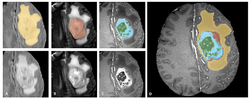
画像パッチは左から右へ以下を示します :

1. T2-FLAIR で見える腫瘍全体 (黄色) (Fig.A)。
2. T2 で見える腫瘍のコア (赤色) (Fig. B)。
3. T1Gd で見える enhancing 腫瘍構造 (ライトブルー)、これはコアの嚢胞 (のうほう) (= cystic) / 壊死 (=necrotic) 成分 (緑色) を取り囲んでいます (Fig. C)。
4. セグメンテーションは 腫瘍部分領域の最終的なラベル (Fig.D) を生成するために組み合わされます : 浮腫 (= edema) (黄色), non-enhancing ソリッドコア (赤色), 嚢胞/壊死コア (緑色), enhancing コア (青色) です。

環境のセットアップ

!python -c "import monai" || pip install -q "monai-weekly[nibabel, tqdm]"
!python -c "import matplotlib" || pip install -q matplotlib
%matplotlib inline

インポートのセットアップ

import os
import shutil
import tempfile
import time
import matplotlib.pyplot as plt
from monai.apps import DecathlonDataset
from monai.config import print_config
from monai.data import DataLoader, decollate_batch
from monai.handlers.utils import from_engine
from monai.losses import DiceLoss
from monai.inferers import sliding_window_inference
from monai.metrics import DiceMetric
from monai.networks.nets import SegResNet
from monai.transforms import (
    Activations,
    Activationsd,
    AsDiscrete,
    AsDiscreted,
    Compose,
    Invertd,
    LoadImaged,
    MapTransform,
    NormalizeIntensityd,
    Orientationd,
    RandFlipd,
    RandScaleIntensityd,
    RandShiftIntensityd,
    RandSpatialCropd,
    Spacingd,
    EnsureTyped,
    EnsureChannelFirstd,
)
from monai.utils import set_determinism

import torch

print_config()

MONAI version: 0.9.1
Numpy version: 1.22.4
Pytorch version: 1.13.0a0+340c412
MONAI flags: HAS_EXT = True, USE_COMPILED = False, USE_META_DICT = False
MONAI rev id: 356d2d2f41b473f588899d705bbc682308cee52c
MONAI __file__: /opt/monai/monai/__init__.py

Optional dependencies:
Pytorch Ignite version: 0.4.9
Nibabel version: 4.0.1
scikit-image version: 0.19.3
Pillow version: 9.0.1
Tensorboard version: 2.9.1
gdown version: 4.5.1
TorchVision version: 0.13.0a0
tqdm version: 4.64.0
lmdb version: 1.3.0
psutil version: 5.9.1
pandas version: 1.3.5
einops version: 0.4.1
transformers version: 4.20.1
mlflow version: 1.27.0
pynrrd version: 0.4.3

For details about installing the optional dependencies, please visit:
    https://docs.monai.io/en/latest/installation.html#installing-the-recommended-dependencies

データディレクトリのセットアップ

MONAI_DATA_DIRECTORY 環境変数でディレクトリを指定できます。これは結果をセーブしてダウンロードを再利用することを可能にします。指定されない場合、一時ディレクトリが使用されます。

directory = os.environ.get("MONAI_DATA_DIRECTORY")
root_dir = tempfile.mkdtemp() if directory is None else directory
print(root_dir)

/workspace/data/medical

再現性のために決定論的訓練を設定する

set_determinism(seed=0)

脳腫瘍のラベルを変換するために新しい変換を定義する

ここでは多クラスラベルを One-Hot 形式のマルチラベルのセグメンテーション・タスクに変換します。

class ConvertToMultiChannelBasedOnBratsClassesd(MapTransform):
    """
    Convert labels to multi channels based on brats classes:
    label 1 is the peritumoral edema
    label 2 is the GD-enhancing tumor
    label 3 is the necrotic and non-enhancing tumor core
    The possible classes are TC (Tumor core), WT (Whole tumor)
    and ET (Enhancing tumor).

    """

    def __call__(self, data):
        d = dict(data)
        for key in self.keys:
            result = []
            # merge label 2 and label 3 to construct TC
            result.append(torch.logical_or(d[key] == 2, d[key] == 3))
            # merge labels 1, 2 and 3 to construct WT
            result.append(
                torch.logical_or(
                    torch.logical_or(d[key] == 2, d[key] == 3), d[key] == 1
                )
            )
            # label 2 is ET
            result.append(d[key] == 2)
            d[key] = torch.stack(result, axis=0).float()
        return d

訓練と検証のための変換のセットアップ

train_transform = Compose(
    [
        # load 4 Nifti images and stack them together
        LoadImaged(keys=["image", "label"]),
        EnsureChannelFirstd(keys="image"),
        EnsureTyped(keys=["image", "label"]),
        ConvertToMultiChannelBasedOnBratsClassesd(keys="label"),
        Orientationd(keys=["image", "label"], axcodes="RAS"),
        Spacingd(
            keys=["image", "label"],
            pixdim=(1.0, 1.0, 1.0),
            mode=("bilinear", "nearest"),
        ),
        RandSpatialCropd(keys=["image", "label"], roi_size=[224, 224, 144], random_size=False),
        RandFlipd(keys=["image", "label"], prob=0.5, spatial_axis=0),
        RandFlipd(keys=["image", "label"], prob=0.5, spatial_axis=1),
        RandFlipd(keys=["image", "label"], prob=0.5, spatial_axis=2),
        NormalizeIntensityd(keys="image", nonzero=True, channel_wise=True),
        RandScaleIntensityd(keys="image", factors=0.1, prob=1.0),
        RandShiftIntensityd(keys="image", offsets=0.1, prob=1.0),
    ]
)
val_transform = Compose(
    [
        LoadImaged(keys=["image", "label"]),
        EnsureChannelFirstd(keys="image"),
        EnsureTyped(keys=["image", "label"]),
        ConvertToMultiChannelBasedOnBratsClassesd(keys="label"),
        Orientationd(keys=["image", "label"], axcodes="RAS"),
        Spacingd(
            keys=["image", "label"],
            pixdim=(1.0, 1.0, 1.0),
            mode=("bilinear", "nearest"),
        ),
        NormalizeIntensityd(keys="image", nonzero=True, channel_wise=True),
    ]
)

DecathlonDataset でデータを素早くロードする

ここではデータセットを自動的にダウンロードして抽出するために DecathlonDataset を使用します。それは MONAI CacheDataset を継承し、より少ないメモリを使用したい場合には、訓練のために N 項目をキャッシュするために cache_num=N を設定して検証のために総ての項目をキャッシュするために default args を使用できます、それはメモリサイズに依存します。

# here we don't cache any data in case out of memory issue
train_ds = DecathlonDataset(
    root_dir=root_dir,
    task="Task01_BrainTumour",
    transform=train_transform,
    section="training",
    download=True,
    cache_rate=0.0,
    num_workers=4,
)
train_loader = DataLoader(train_ds, batch_size=1, shuffle=True, num_workers=4)
val_ds = DecathlonDataset(
    root_dir=root_dir,
    task="Task01_BrainTumour",
    transform=val_transform,
    section="validation",
    download=False,
    cache_rate=0.0,
    num_workers=4,
)
val_loader = DataLoader(val_ds, batch_size=1, shuffle=False, num_workers=4)

Verified 'Task01_BrainTumour.tar', md5: 240a19d752f0d9e9101544901065d872.
File exists: /workspace/data/medical/Task01_BrainTumour.tar, skipped downloading.
Non-empty folder exists in /workspace/data/medical/Task01_BrainTumour, skipped extracting.

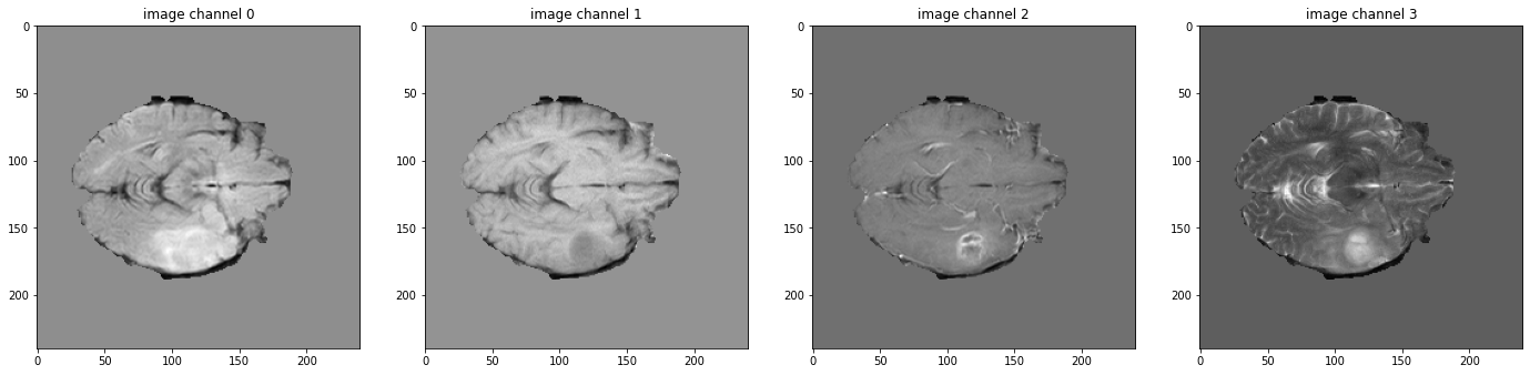
データ shape を確認して可視化する

# pick one image from DecathlonDataset to visualize and check the 4 channels
val_data_example = val_ds[2]
print(f"image shape: {val_data_example['image'].shape}")
plt.figure("image", (24, 6))
for i in range(4):
    plt.subplot(1, 4, i + 1)
    plt.title(f"image channel {i}")
    plt.imshow(val_data_example["image"][i, :, :, 60].detach().cpu(), cmap="gray")
plt.show()
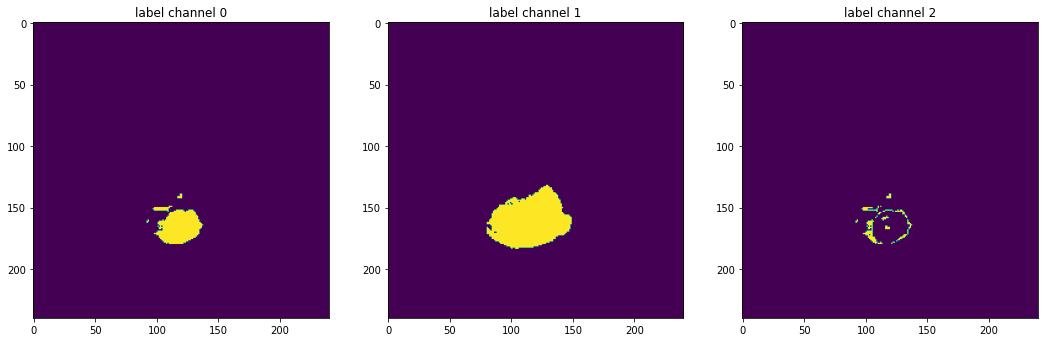
# also visualize the 3 channels label corresponding to this image
print(f"label shape: {val_data_example['label'].shape}")
plt.figure("label", (18, 6))
for i in range(3):
    plt.subplot(1, 3, i + 1)
    plt.title(f"label channel {i}")
    plt.imshow(val_data_example["label"][i, :, :, 60].detach().cpu())
plt.show()

image shape: torch.Size([4, 240, 240, 155])

モデル, 損失, Optimizer を作成する

max_epochs = 300
val_interval = 1
VAL_AMP = True

# standard PyTorch program style: create SegResNet, DiceLoss and Adam optimizer
device = torch.device("cuda:0")
model = SegResNet(
    blocks_down=[1, 2, 2, 4],
    blocks_up=[1, 1, 1],
    init_filters=16,
    in_channels=4,
    out_channels=3,
    dropout_prob=0.2,
).to(device)
loss_function = DiceLoss(smooth_nr=0, smooth_dr=1e-5, squared_pred=True, to_onehot_y=False, sigmoid=True)
optimizer = torch.optim.Adam(model.parameters(), 1e-4, weight_decay=1e-5)
lr_scheduler = torch.optim.lr_scheduler.CosineAnnealingLR(optimizer, T_max=max_epochs)

dice_metric = DiceMetric(include_background=True, reduction="mean")
dice_metric_batch = DiceMetric(include_background=True, reduction="mean_batch")

post_trans = Compose(
    [Activations(sigmoid=True), AsDiscrete(threshold=0.5)]
)


# define inference method
def inference(input):

    def _compute(input):
        return sliding_window_inference(
            inputs=input,
            roi_size=(240, 240, 160),
            sw_batch_size=1,
            predictor=model,
            overlap=0.5,
        )

    if VAL_AMP:
        with torch.cuda.amp.autocast():
            return _compute(input)
    else:
        return _compute(input)


# use amp to accelerate training
scaler = torch.cuda.amp.GradScaler()
# enable cuDNN benchmark
torch.backends.cudnn.benchmark = True

典型的な PyTorch 訓練プロセスの実行

best_metric = -1
best_metric_epoch = -1
best_metrics_epochs_and_time = [[], [], []]
epoch_loss_values = []
metric_values = []
metric_values_tc = []
metric_values_wt = []
metric_values_et = []

total_start = time.time()
for epoch in range(max_epochs):
    epoch_start = time.time()
    print("-" * 10)
    print(f"epoch {epoch + 1}/{max_epochs}")
    model.train()
    epoch_loss = 0
    step = 0
    for batch_data in train_loader:
        step_start = time.time()
        step += 1
        inputs, labels = (
            batch_data["image"].to(device),
            batch_data["label"].to(device),
        )
        optimizer.zero_grad()
        with torch.cuda.amp.autocast():
            outputs = model(inputs)
            loss = loss_function(outputs, labels)
        scaler.scale(loss).backward()
        scaler.step(optimizer)
        scaler.update()
        epoch_loss += loss.item()
        print(
            f"{step}/{len(train_ds) // train_loader.batch_size}"
            f", train_loss: {loss.item():.4f}"
            f", step time: {(time.time() - step_start):.4f}"
        )
    lr_scheduler.step()
    epoch_loss /= step
    epoch_loss_values.append(epoch_loss)
    print(f"epoch {epoch + 1} average loss: {epoch_loss:.4f}")

    if (epoch + 1) % val_interval == 0:
        model.eval()
        with torch.no_grad():

            for val_data in val_loader:
                val_inputs, val_labels = (
                    val_data["image"].to(device),
                    val_data["label"].to(device),
                )
                val_outputs = inference(val_inputs)
                val_outputs = [post_trans(i) for i in decollate_batch(val_outputs)]
                dice_metric(y_pred=val_outputs, y=val_labels)
                dice_metric_batch(y_pred=val_outputs, y=val_labels)

            metric = dice_metric.aggregate().item()
            metric_values.append(metric)
            metric_batch = dice_metric_batch.aggregate()
            metric_tc = metric_batch[0].item()
            metric_values_tc.append(metric_tc)
            metric_wt = metric_batch[1].item()
            metric_values_wt.append(metric_wt)
            metric_et = metric_batch[2].item()
            metric_values_et.append(metric_et)
            dice_metric.reset()
            dice_metric_batch.reset()

            if metric > best_metric:
                best_metric = metric
                best_metric_epoch = epoch + 1
                best_metrics_epochs_and_time[0].append(best_metric)
                best_metrics_epochs_and_time[1].append(best_metric_epoch)
                best_metrics_epochs_and_time[2].append(time.time() - total_start)
                torch.save(
                    model.state_dict(),
                    os.path.join(root_dir, "best_metric_model.pth"),
                )
                print("saved new best metric model")
            print(
                f"current epoch: {epoch + 1} current mean dice: {metric:.4f}"
                f" tc: {metric_tc:.4f} wt: {metric_wt:.4f} et: {metric_et:.4f}"
                f"\nbest mean dice: {best_metric:.4f}"
                f" at epoch: {best_metric_epoch}"
            )
    print(f"time consuming of epoch {epoch + 1} is: {(time.time() - epoch_start):.4f}")
total_time = time.time() - total_start

print(f"train completed, best_metric: {best_metric:.4f} at epoch: {best_metric_epoch}, total time: {total_time}.")

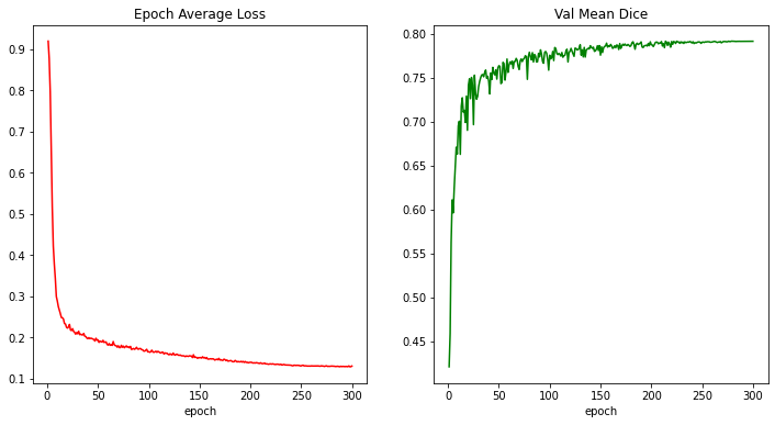
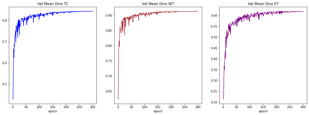
train completed, best_metric: 0.7914 at epoch: 279, total time: 90155.70936012268.

損失とメトリックのプロット

plt.figure("train", (12, 6))
plt.subplot(1, 2, 1)
plt.title("Epoch Average Loss")
x = [i + 1 for i in range(len(epoch_loss_values))]
y = epoch_loss_values
plt.xlabel("epoch")
plt.plot(x, y, color="red")
plt.subplot(1, 2, 2)
plt.title("Val Mean Dice")
x = [val_interval * (i + 1) for i in range(len(metric_values))]
y = metric_values
plt.xlabel("epoch")
plt.plot(x, y, color="green")
plt.show()

plt.figure("train", (18, 6))
plt.subplot(1, 3, 1)
plt.title("Val Mean Dice TC")
x = [val_interval * (i + 1) for i in range(len(metric_values_tc))]
y = metric_values_tc
plt.xlabel("epoch")
plt.plot(x, y, color="blue")
plt.subplot(1, 3, 2)
plt.title("Val Mean Dice WT")
x = [val_interval * (i + 1) for i in range(len(metric_values_wt))]
y = metric_values_wt
plt.xlabel("epoch")
plt.plot(x, y, color="brown")
plt.subplot(1, 3, 3)
plt.title("Val Mean Dice ET")
x = [val_interval * (i + 1) for i in range(len(metric_values_et))]
y = metric_values_et
plt.xlabel("epoch")
plt.plot(x, y, color="purple")
plt.show()

入力画像とラベルでベストモデル出力を確認する

model.load_state_dict(
    torch.load(os.path.join(root_dir, "best_metric_model.pth"))
)
model.eval()
with torch.no_grad():
    # select one image to evaluate and visualize the model output
    val_input = val_ds[6]["image"].unsqueeze(0).to(device)
    roi_size = (128, 128, 64)
    sw_batch_size = 4
    val_output = inference(val_input)
    val_output = post_trans(val_output[0])
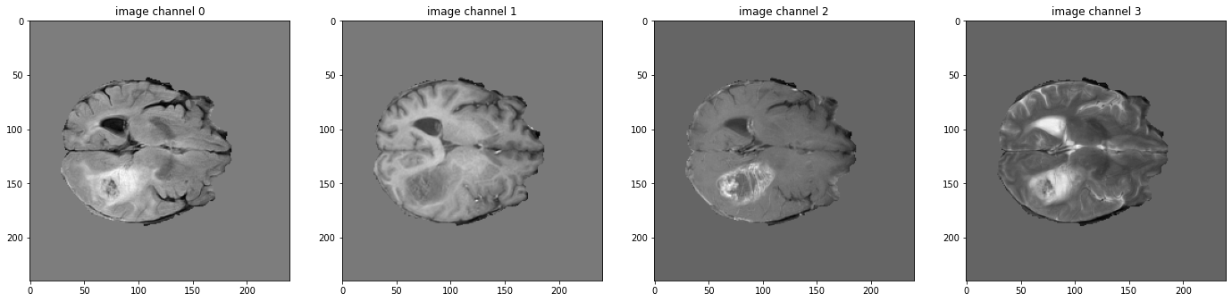
    plt.figure("image", (24, 6))
    for i in range(4):
        plt.subplot(1, 4, i + 1)
        plt.title(f"image channel {i}")
        plt.imshow(val_ds[6]["image"][i, :, :, 70].detach().cpu(), cmap="gray")
    plt.show()
    # visualize the 3 channels label corresponding to this image
    plt.figure("label", (18, 6))
    for i in range(3):
        plt.subplot(1, 3, i + 1)
        plt.title(f"label channel {i}")
        plt.imshow(val_ds[6]["label"][i, :, :, 70].detach().cpu())
    plt.show()
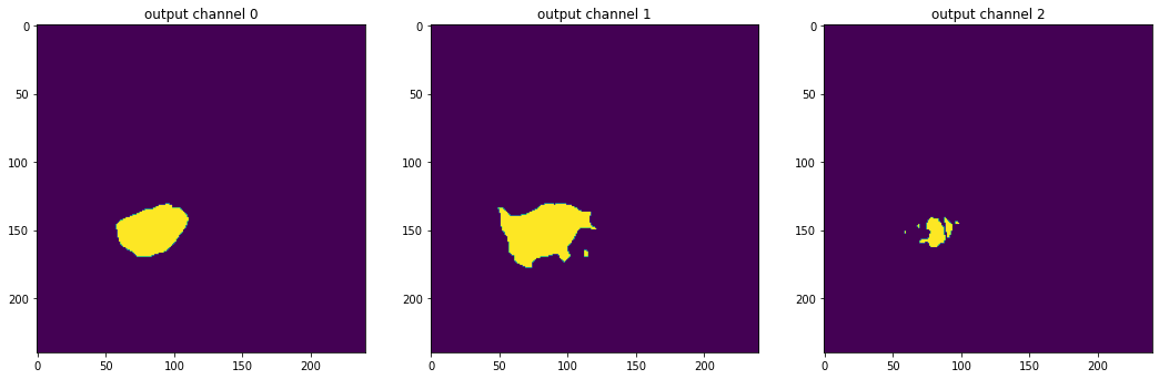
    # visualize the 3 channels model output corresponding to this image
    plt.figure("output", (18, 6))
    for i in range(3):
        plt.subplot(1, 3, i + 1)
        plt.title(f"output channel {i}")
        plt.imshow(val_output[i, :, :, 70].detach().cpu())
    plt.show()

元の画像 spacings 上の評価

val_org_transforms = Compose(
    [
        LoadImaged(keys=["image", "label"]),
        EnsureChannelFirstd(keys=["image"]),
        ConvertToMultiChannelBasedOnBratsClassesd(keys="label"),
        Orientationd(keys=["image"], axcodes="RAS"),
        Spacingd(keys=["image"], pixdim=(1.0, 1.0, 1.0), mode="bilinear"),
        NormalizeIntensityd(keys="image", nonzero=True, channel_wise=True),
    ]
)

val_org_ds = DecathlonDataset(
    root_dir=root_dir,
    task="Task01_BrainTumour",
    transform=val_org_transforms,
    section="validation",
    download=False,
    num_workers=4,
    cache_num=0,
)
val_org_loader = DataLoader(val_org_ds, batch_size=1, shuffle=False, num_workers=4)

post_transforms = Compose([
    Invertd(
        keys="pred",
        transform=val_org_transforms,
        orig_keys="image",
        meta_keys="pred_meta_dict",
        orig_meta_keys="image_meta_dict",
        meta_key_postfix="meta_dict",
        nearest_interp=False,
        to_tensor=True,
        device="cpu",
    ),
    Activationsd(keys="pred", sigmoid=True),
    AsDiscreted(keys="pred", threshold=0.5),
])

model.load_state_dict(torch.load(
    os.path.join(root_dir, "best_metric_model.pth")))
model.eval()

with torch.no_grad():
    for val_data in val_org_loader:
        val_inputs = val_data["image"].to(device)
        val_data["pred"] = inference(val_inputs)
        val_data = [post_transforms(i) for i in decollate_batch(val_data)]
        val_outputs, val_labels = from_engine(["pred", "label"])(val_data)
        dice_metric(y_pred=val_outputs, y=val_labels)
        dice_metric_batch(y_pred=val_outputs, y=val_labels)

    metric_org = dice_metric.aggregate().item()
    metric_batch_org = dice_metric_batch.aggregate()

    dice_metric.reset()
    dice_metric_batch.reset()

metric_tc, metric_wt, metric_et = metric_batch_org[0].item(), metric_batch_org[1].item(), metric_batch_org[2].item()

print("Metric on original image spacing: ", metric_org)
print(f"metric_tc: {metric_tc:.4f}")
print(f"metric_wt: {metric_wt:.4f}")
print(f"metric_et: {metric_et:.4f}")

Metric on original image spacing:  0.7912478446960449
metric_tc: 0.8422
metric_wt: 0.9129
metric_et: 0.6187

データディレクトリのクリーンアップ

一時ディレクトリが使用された場合ディレクトリを削除します。

if directory is None:
    shutil.rmtree(root_dir)

以上