ホーム » 「PyOD 0.8」タグがついた投稿

タグアーカイブ: PyOD 0.8

PyOD 0.8 : Examples : AutoEncoder

06/28/2021

PyOD 0.8 : Examples : AutoEncoder (解説)
翻訳 : (株)クラスキャットセールスインフォメーション
作成日時 : 06/28/2021 (0.8.9)

* 本ページは、PyOD の以下のドキュメントとサンプルを参考にして作成しています：

* ご自由にリンクを張って頂いてかまいませんが、sales-info@classcat.com までご一報いただけると嬉しいです。

PyOD 0.8 : Examples : AutoEncoder

完全なサンプル : examples/auto_encoder_example.py

合成データの生成

pyod.utils.data.generate_data() でサンプルデータを生成します :

from pyod.utils.data import generate_data

contamination = 0.1  # percentage of outliers
n_train = 20000  # number of training points
n_test = 2000  # number of testing points
n_features = 300  # number of features

# Generate sample data
X_train, y_train, X_test, y_test = generate_data(
    n_train=n_train,
    n_test=n_test,
    n_features=n_features,
    contamination=contamination,
    random_state=42)

X_train, y_train の shape と値を確認します :

print(X_train.shape)
print(y_train.shape)

(20000, 300)
(20000,)

X_train[:10]

array([[6.43365854, 5.5091683 , 5.04469788, ..., 4.98920813, 6.08796866,
        5.65703627],
       [6.98114644, 4.97019307, 7.24011768, ..., 4.13407401, 4.17437525,
        7.14246591],
       [6.96879306, 5.29747338, 5.29666367, ..., 5.97531553, 6.40414268,
        5.8399228 ],
       ...,
       [5.13676552, 6.62890142, 6.14075622, ..., 5.42330645, 5.68013833,
        7.49193446],
       [6.09141558, 5.30143243, 7.09624952, ..., 6.32592813, 7.31717914,
        7.4945297 ],
       [5.74924769, 6.76427622, 7.10854915, ..., 6.38070765, 6.23367069,
        6.3011638 ]])

y_train[:10]

array([0., 0., 0., 0., 0., 0., 0., 0., 0., 0.])

モデル訓練

pyod.models.auto_encoder.AutoEncoder 検出器をインポートして初期化し、そしてモデルを適合させます。

オートエンコーダ (AE) は有用なデータ表現を教師なしで学習するためのニューラルネットワークの一種です。PCA と同様に、再構築エラーを計算することによりデータの外れ値オブジェクトを検出するために使用できるでしょう。

参照 :

Charu C Aggarwal. Outlier analysis. In Data mining, 75–79. Springer, 2015.

from pyod.models.auto_encoder import AutoEncoder

# train AutoEncoder detector
clf_name = 'AutoEncoder'
clf = AutoEncoder(epochs=30, contamination=contamination)
clf.fit(X_train)

Model: "sequential"
_________________________________________________________________
Layer (type)                 Output Shape              Param #   
=================================================================
dense (Dense)                (None, 300)               90300     
_________________________________________________________________
dropout (Dropout)            (None, 300)               0         
_________________________________________________________________
dense_1 (Dense)              (None, 300)               90300     
_________________________________________________________________
dropout_1 (Dropout)          (None, 300)               0         
_________________________________________________________________
dense_2 (Dense)              (None, 64)                19264     
_________________________________________________________________
dropout_2 (Dropout)          (None, 64)                0         
_________________________________________________________________
dense_3 (Dense)              (None, 32)                2080      
_________________________________________________________________
dropout_3 (Dropout)          (None, 32)                0         
_________________________________________________________________
dense_4 (Dense)              (None, 32)                1056      
_________________________________________________________________
dropout_4 (Dropout)          (None, 32)                0         
_________________________________________________________________
dense_5 (Dense)              (None, 64)                2112      
_________________________________________________________________
dropout_5 (Dropout)          (None, 64)                0         
_________________________________________________________________
dense_6 (Dense)              (None, 300)               19500     
=================================================================
Total params: 224,612
Trainable params: 224,612
Non-trainable params: 0
_________________________________________________________________
None
Epoch 1/30
563/563 [==============================] - 2s 3ms/step - loss: 3.9799 - val_loss: 1.6536
Epoch 2/30
563/563 [==============================] - 1s 2ms/step - loss: 1.3378 - val_loss: 1.2611
Epoch 3/30
563/563 [==============================] - 1s 2ms/step - loss: 1.1653 - val_loss: 1.1830
Epoch 4/30
563/563 [==============================] - 1s 2ms/step - loss: 1.1163 - val_loss: 1.1421
Epoch 5/30
563/563 [==============================] - 1s 2ms/step - loss: 1.0902 - val_loss: 1.1188
Epoch 6/30
563/563 [==============================] - 1s 2ms/step - loss: 1.0745 - val_loss: 1.1108
Epoch 7/30
563/563 [==============================] - 1s 2ms/step - loss: 1.0609 - val_loss: 1.0937
Epoch 8/30
563/563 [==============================] - 1s 2ms/step - loss: 1.0519 - val_loss: 1.0851
Epoch 9/30
563/563 [==============================] - 1s 2ms/step - loss: 1.0439 - val_loss: 1.0823
Epoch 10/30
563/563 [==============================] - 1s 2ms/step - loss: 1.0372 - val_loss: 1.0715
Epoch 11/30
563/563 [==============================] - 1s 2ms/step - loss: 1.0309 - val_loss: 1.0658
Epoch 12/30
563/563 [==============================] - 1s 2ms/step - loss: 1.0247 - val_loss: 1.0612
Epoch 13/30
563/563 [==============================] - 1s 2ms/step - loss: 1.0193 - val_loss: 1.0576
Epoch 14/30
563/563 [==============================] - 1s 2ms/step - loss: 1.0158 - val_loss: 1.0543
Epoch 15/30
563/563 [==============================] - 1s 2ms/step - loss: 1.0129 - val_loss: 1.0523
Epoch 16/30
563/563 [==============================] - 1s 2ms/step - loss: 1.0103 - val_loss: 1.0495
Epoch 17/30
563/563 [==============================] - 1s 2ms/step - loss: 1.0081 - val_loss: 1.0476
Epoch 18/30
563/563 [==============================] - 1s 2ms/step - loss: 1.0062 - val_loss: 1.0460
Epoch 19/30
563/563 [==============================] - 1s 2ms/step - loss: 1.0045 - val_loss: 1.0445
Epoch 20/30
563/563 [==============================] - 1s 2ms/step - loss: 1.0031 - val_loss: 1.0433
Epoch 21/30
563/563 [==============================] - 1s 2ms/step - loss: 1.0019 - val_loss: 1.0422
Epoch 22/30
563/563 [==============================] - 1s 2ms/step - loss: 1.0008 - val_loss: 1.0413
Epoch 23/30
563/563 [==============================] - 1s 2ms/step - loss: 1.0001 - val_loss: 1.0405
Epoch 24/30
563/563 [==============================] - 1s 2ms/step - loss: 0.9993 - val_loss: 1.0399
Epoch 25/30
563/563 [==============================] - 1s 2ms/step - loss: 0.9987 - val_loss: 1.0394
Epoch 26/30
563/563 [==============================] - 1s 2ms/step - loss: 0.9982 - val_loss: 1.0389
Epoch 27/30
563/563 [==============================] - 1s 2ms/step - loss: 0.9978 - val_loss: 1.0386
Epoch 28/30
563/563 [==============================] - 1s 2ms/step - loss: 0.9975 - val_loss: 1.0383
Epoch 29/30
563/563 [==============================] - 1s 2ms/step - loss: 0.9972 - val_loss: 1.0380
Epoch 30/30
563/563 [==============================] - 1s 2ms/step - loss: 0.9969 - val_loss: 1.0378

AutoEncoder(batch_size=32, contamination=0.1, dropout_rate=0.2, epochs=30,
      hidden_activation='relu', hidden_neurons=[64, 32, 32, 64],
      l2_regularizer=0.1,
      loss=,
      optimizer='adam', output_activation='sigmoid', preprocessing=True,
      random_state=None, validation_size=0.1, verbose=1)

訓練データの予測ラベルと外れ値スコアを取得します :

y_train_pred = clf.labels_  # binary labels (0: inliers, 1: outliers)
y_train_scores = clf.decision_scores_  # raw outlier scores

y_train_pred

array([0, 0, 0, ..., 1, 1, 1])

y_train_scores[:10]

array([7.71661709, 8.3933272 , 8.03062351, 8.3012123 , 7.29930043,
       7.8202035 , 8.25040261, 7.89435037, 8.68701496, 7.54829144])

予測と評価

先に正解ラベルを確認しておきます :

y_test

array([0., array([0., 0., 0., ..., 1., 1., 1.])

テストデータ上で予測を行ないます :

y_test_pred = clf.predict(X_test)  # outlier labels (0 or 1)
y_test_scores = clf.decision_function(X_test)  # outlier scores

y_test_pred

array([0, 0, 0, ..., 1, 1, 1])

y_test_scores[:10]

array([7.88748478, 7.4678574 , 7.68665623, 7.7947202 , 7.81147175,
       7.44892412, 7.35455911, 7.74632114, 7.46644309, 8.08000442])

ROC と Precision @ Rank n pyod.utils.data.evaluate_print() を使用して予測を評価します。

from pyod.utils.data import evaluate_print
# evaluate and print the results
print("\nOn Training Data:")
evaluate_print(clf_name, y_train, y_train_scores)
print("\nOn Test Data:")
evaluate_print(clf_name, y_test, y_test_scores)

On Training Data:
AutoEncoder ROC:1.0, precision @ rank n:1.0

On Test Data:
AutoEncoder ROC:1.0, precision @ rank n:1.0

以上

PyOD 0.8 : Examples : Isolation Forest

06/28/2021

PyOD 0.8 : Examples : Isolation Forest (解説)
翻訳 : (株)クラスキャットセールスインフォメーション
作成日時 : 06/28/2021 (0.8.9)

* 本ページは、PyOD の以下のドキュメントとサンプルを参考にして作成しています：

* ご自由にリンクを張って頂いてかまいませんが、sales-info@classcat.com までご一報いただけると嬉しいです。

★ 無料 Web セミナー開催中 ★ クラスキャット主催人工知能 & ビジネス Web セミナー

人工知能とビジネスをテーマに WEB セミナーを定期的に開催しています。
スケジュールは弊社公式 Web サイトでご確認頂けます。

お住まいの地域に関係なく Web ブラウザからご参加頂けます。事前登録 が必要ですのでご注意ください。
ウェビナー運用には弊社製品「ClassCat® Webinar」を利用しています。

クラスキャットは人工知能・テレワークに関する各種サービスを提供しております :

人工知能研究開発支援	人工知能研修サービス	テレワーク & オンライン授業を支援
PoC(概念実証)を失敗させないための支援 (本支援はセミナーに参加しアンケートに回答した方を対象としています。)

◆ お問合せ : 本件に関するお問い合わせ先は下記までお願いいたします。

株式会社クラスキャット セールス・マーケティング本部セールス・インフォメーション

E-Mail：sales-info@classcat.com ; WebSite: https://www.classcat.com/ ; Facebook

PyOD 0.8 : Examples : Isolation Forest

完全なサンプル : examples/iforest_example.py

合成データの生成と可視化

pyod.utils.data.generate_data() でサンプルデータを生成します :

from pyod.utils.data import generate_data

contamination = 0.1  # percentage of outliers
n_train = 200  # number of training points
n_test = 100  # number of testing points

X_train, y_train, X_test, y_test = generate_data(
    n_train=n_train, n_test=n_test,
    n_features=2,
    contamination=contamination,
    random_state=42
)

X_train, y_train の shape と値を確認します :

print(X_train.shape)
print(y_train.shape)

(200, 2)
(200,)

X_train[:10]

array([[6.43365854, 5.5091683 ],
       [5.04469788, 7.70806466],
       [5.92453568, 5.25921966],
       [5.29399075, 5.67126197],
       [5.61509076, 6.1309285 ],
       [6.18590347, 6.09410578],
       [7.16630941, 7.22719133],
       [4.05470826, 6.48127032],
       [5.79978164, 5.86930893],
       [4.82256361, 7.18593123]])

y_train[:200]

array([0., 0., 0., 0., 0., 0., 0., 0., 0., 0., 0., 0., 0., 0., 0., 0., 0.,
       0., 0., 0., 0., 0., 0., 0., 0., 0., 0., 0., 0., 0., 0., 0., 0., 0.,
       0., 0., 0., 0., 0., 0., 0., 0., 0., 0., 0., 0., 0., 0., 0., 0., 0.,
       0., 0., 0., 0., 0., 0., 0., 0., 0., 0., 0., 0., 0., 0., 0., 0., 0.,
       0., 0., 0., 0., 0., 0., 0., 0., 0., 0., 0., 0., 0., 0., 0., 0., 0.,
       0., 0., 0., 0., 0., 0., 0., 0., 0., 0., 0., 0., 0., 0., 0., 0., 0.,
       0., 0., 0., 0., 0., 0., 0., 0., 0., 0., 0., 0., 0., 0., 0., 0., 0.,
       0., 0., 0., 0., 0., 0., 0., 0., 0., 0., 0., 0., 0., 0., 0., 0., 0.,
       0., 0., 0., 0., 0., 0., 0., 0., 0., 0., 0., 0., 0., 0., 0., 0., 0.,
       0., 0., 0., 0., 0., 0., 0., 0., 0., 0., 0., 0., 0., 0., 0., 0., 0.,
       0., 0., 0., 0., 0., 0., 0., 0., 0., 0., 1., 1., 1., 1., 1., 1., 1.,
       1., 1., 1., 1., 1., 1., 1., 1., 1., 1., 1., 1., 1.])

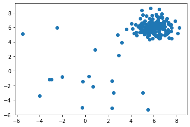
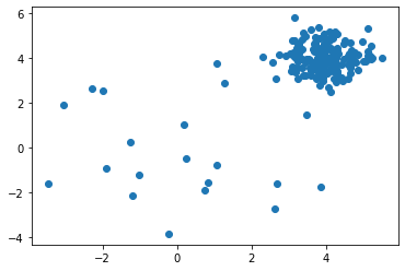
X_train の分布を可視化します :

import matplotlib.pyplot as plt
 
plt.scatter(X_train[:, 0], X_train[:, 1])

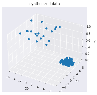
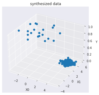
訓練データを可視化します :

import seaborn as sns
sns.set_style("dark")

from mpl_toolkits.mplot3d import Axes3D

X0 = X_train[:, 0]
X1 = X_train[:, 1]
Y = y_train

fig = plt.figure()
ax = Axes3D(fig)

ax.set_title("synthesized data")
 
ax.set_xlabel("X0")
ax.set_ylabel("X1")
ax.set_zlabel("Y")
 
ax.plot(X0, X1, Y, marker="o",linestyle='None')

モデル訓練

pyod.models.iforest.IForest 検出器をインポートして初期化し、そしてモデルを適合させます。

scikit-learn Isolation Forest のより多くの機能を持つラッパーです。

IsolationForest は、特徴をランダムに選択してから選択された特徴の最大値と最小値の間の分割値 (= split value) をランダムに選択することにより観測を「分離 (= isolate)」します。

参照 :

Fei Tony Liu, Kai Ming Ting, and Zhi-Hua Zhou. Isolation forest. In Data Mining, 2008. ICDM’08. Eighth IEEE International Conference on, 413–422. IEEE, 2008.
Fei Tony Liu, Kai Ming Ting, and Zhi-Hua Zhou. Isolation-based anomaly detection. ACM Transactions on Knowledge Discovery from Data (TKDD), 6(1):3, 2012.

再帰的分割 (= partitioning) は木構造で表されますので、サンプルを分離するために必要な分割の数はルートノードから終端ノードへのパスの長さに等しいです。

そのようなランダムツリーの森 (= forest) に渡り平均された、このパスの長さは正常性と決定関数の尺度です。

ランダム分割は異常値のためには著しく短いパスを生成します。そのため、ランダムツリーの森が特定のサンプルのために短いパスの長さを集合的に生成するとき、それらは異常である可能性が高くなります。

from pyod.models.iforest import IForest

clf_name = 'IForest'
clf = IForest()
clf.fit(X_train)

IForest(behaviour='old', bootstrap=False, contamination=0.1, max_features=1.0,
    max_samples='auto', n_estimators=100, n_jobs=1, random_state=None,
    verbose=0)

訓練データの予測ラベルと外れ値スコアを取得します :

y_train_pred = clf.labels_  # binary labels (0: inliers, 1: outliers)
y_train_scores = clf.decision_scores_  # raw outlier scores

y_train_pred

array([0, 0, 0, 0, 0, 0, 0, 0, 0, 0, 0, 0, 0, 0, 0, 0, 0, 0, 0, 0, 0, 0,
       0, 0, 0, 0, 0, 0, 0, 0, 0, 0, 0, 0, 0, 0, 0, 0, 0, 0, 0, 0, 0, 0,
       0, 0, 0, 0, 0, 0, 0, 0, 0, 0, 0, 0, 0, 0, 0, 0, 0, 0, 0, 0, 0, 0,
       0, 0, 0, 0, 0, 0, 0, 0, 0, 0, 0, 0, 0, 0, 0, 0, 0, 0, 0, 0, 0, 0,
       0, 0, 0, 0, 1, 0, 0, 0, 0, 0, 0, 1, 0, 0, 0, 0, 0, 0, 0, 0, 0, 0,
       0, 0, 0, 0, 0, 0, 0, 0, 0, 0, 0, 0, 0, 0, 0, 0, 0, 0, 0, 0, 0, 0,
       0, 0, 0, 0, 0, 0, 0, 0, 0, 0, 0, 0, 0, 0, 0, 0, 0, 0, 0, 0, 0, 0,
       0, 0, 0, 0, 0, 0, 0, 0, 0, 0, 1, 0, 0, 0, 0, 0, 0, 0, 0, 0, 0, 0,
       0, 0, 0, 0, 1, 1, 1, 1, 1, 0, 1, 1, 1, 1, 0, 1, 1, 1, 1, 1, 1, 1,
       0, 1])

y_train_scores[-40:]

array([-0.1846575 , -0.17420279, -0.16454624, -0.18313387,  0.00184097,
       -0.16721463, -0.20881165, -0.12698201, -0.20432723, -0.19229842,
       -0.18207002, -0.10462056, -0.21048142, -0.17633758, -0.18314583,
       -0.17556592, -0.17987594, -0.20584378, -0.19802026, -0.15455344,
        0.03418722,  0.05486257,  0.06756084,  0.04571578,  0.07418781,
       -0.01109817,  0.03804931,  0.05553404,  0.11342275,  0.03541737,
       -0.06930148,  0.04314033,  0.20286855,  0.08323074,  0.09318281,
        0.14768482,  0.13077218,  0.03692   , -0.03166733,  0.11722839])

予測と評価

先に正解ラベルを確認しておきます :

y_test

array([0., array([0., 0., 0., 0., 0., 0., 0., 0., 0., 0., 0., 0., 0., 0., 0., 0., 0.,
       0., 0., 0., 0., 0., 0., 0., 0., 0., 0., 0., 0., 0., 0., 0., 0., 0.,
       0., 0., 0., 0., 0., 0., 0., 0., 0., 0., 0., 0., 0., 0., 0., 0., 0.,
       0., 0., 0., 0., 0., 0., 0., 0., 0., 0., 0., 0., 0., 0., 0., 0., 0.,
       0., 0., 0., 0., 0., 0., 0., 0., 0., 0., 0., 0., 0., 0., 0., 0., 0.,
       0., 0., 0., 0., 0., 1., 1., 1., 1., 1., 1., 1., 1., 1., 1.])

テストデータ上で予測を行ないます :

y_test_pred = clf.predict(X_test)  # outlier labels (0 or 1)
y_test_scores = clf.decision_function(X_test)  # outlier scores

y_test_pred

aarray([0, 0, 0, 0, 0, 0, 0, 0, 0, 0, 0, 0, 0, 0, 0, 0, 0, 0, 0, 0, 0, 0,
       0, 0, 0, 0, 0, 0, 0, 0, 0, 0, 0, 0, 0, 0, 0, 0, 0, 0, 0, 0, 0, 0,
       0, 0, 0, 0, 0, 0, 0, 0, 0, 0, 0, 0, 0, 0, 0, 0, 0, 0, 0, 0, 0, 0,
       0, 0, 0, 0, 0, 0, 0, 0, 0, 0, 0, 0, 0, 0, 0, 0, 0, 0, 0, 0, 0, 0,
       0, 0, 1, 1, 1, 1, 0, 1, 1, 1, 1, 1])

y_test_scores[-40:]

array([-0.12997412, -0.20032257, -0.17450527, -0.17089002, -0.10767756,
       -0.13952181, -0.01800938, -0.14394372, -0.07613799, -0.15948458,
       -0.19488334, -0.14925167, -0.20239421, -0.09349558, -0.1980245 ,
       -0.10904396, -0.19059866, -0.00824005, -0.20500567, -0.1781156 ,
       -0.1023197 , -0.20947508, -0.19867088, -0.13209401, -0.11648015,
       -0.02002286, -0.17712404, -0.0594405 , -0.20782814, -0.20041835,
        0.0692155 ,  0.08597497,  0.0822211 ,  0.1060188 , -0.01362171,
        0.00519536,  0.08507602,  0.11226714,  0.07143067,  0.07464685])

ROC と Precision @ Rank n pyod.utils.data.evaluate_print() を使用して予測を評価します。

from pyod.utils.data import evaluate_print
# evaluate and print the results
print("\nOn Training Data:")
evaluate_print(clf_name, y_train, y_train_scores)
print("\nOn Test Data:")
evaluate_print(clf_name, y_test, y_test_scores)

On Training Data:
IForest ROC:0.9944, precision @ rank n:0.85

On Test Data:
IForest ROC:0.9978, precision @ rank n:0.9

総ての examples に含まれる visualize 関数により可視化を生成します :

from pyod.utils.example import visualize
 
visualize(clf_name, X_train, y_train, X_test, y_test, y_train_pred,
          y_test_pred, show_figure=True, save_figure=False)

以上

PyOD 0.8 : Examples : 局所外れ値因子 (LOF)

06/28/2021

PyOD 0.8 : Examples : 局所外れ値因子 (LOF) (解説)
翻訳 : (株)クラスキャットセールスインフォメーション
作成日時 : 06/28/2021 (0.8.9)

* 本ページは、PyOD の以下のドキュメントとサンプルを参考にして作成しています：

* ご自由にリンクを張って頂いてかまいませんが、sales-info@classcat.com までご一報いただけると嬉しいです。

★ 無料 Web セミナー開催中 ★ クラスキャット主催人工知能 & ビジネス Web セミナー

人工知能とビジネスをテーマに WEB セミナーを定期的に開催しています。
スケジュールは弊社公式 Web サイトでご確認頂けます。

お住まいの地域に関係なく Web ブラウザからご参加頂けます。事前登録 が必要ですのでご注意ください。
ウェビナー運用には弊社製品「ClassCat® Webinar」を利用しています。

クラスキャットは人工知能・テレワークに関する各種サービスを提供しております :

人工知能研究開発支援	人工知能研修サービス	テレワーク & オンライン授業を支援
PoC(概念実証)を失敗させないための支援 (本支援はセミナーに参加しアンケートに回答した方を対象としています。)

◆ お問合せ : 本件に関するお問い合わせ先は下記までお願いいたします。

株式会社クラスキャット セールス・マーケティング本部セールス・インフォメーション

E-Mail：sales-info@classcat.com ; WebSite: https://www.classcat.com/ ; Facebook

PyOD 0.8 : Examples : 局所外れ値因子 (LOF)

完全なサンプル : examples/lof_example.py

合成データの生成と可視化

pyod.utils.data.generate_data() でサンプルデータを生成します :

from pyod.utils.data import generate_data

contamination = 0.1  # percentage of outliers
n_train = 200  # number of training points
n_test = 100  # number of testing points

X_train, y_train, X_test, y_test = generate_data(
    n_train=n_train, n_test=n_test,
    n_features=2,
    contamination=contamination,
    random_state=42
)

X_train, y_train の shape と値を確認します :

print(X_train.shape)
print(y_train.shape)

(200, 2)
(200,)

X_train[:10]

array([[6.43365854, 5.5091683 ],
       [5.04469788, 7.70806466],
       [5.92453568, 5.25921966],
       [5.29399075, 5.67126197],
       [5.61509076, 6.1309285 ],
       [6.18590347, 6.09410578],
       [7.16630941, 7.22719133],
       [4.05470826, 6.48127032],
       [5.79978164, 5.86930893],
       [4.82256361, 7.18593123]])

y_train[:200]

array([0., 0., 0., 0., 0., 0., 0., 0., 0., 0., 0., 0., 0., 0., 0., 0., 0.,
       0., 0., 0., 0., 0., 0., 0., 0., 0., 0., 0., 0., 0., 0., 0., 0., 0.,
       0., 0., 0., 0., 0., 0., 0., 0., 0., 0., 0., 0., 0., 0., 0., 0., 0.,
       0., 0., 0., 0., 0., 0., 0., 0., 0., 0., 0., 0., 0., 0., 0., 0., 0.,
       0., 0., 0., 0., 0., 0., 0., 0., 0., 0., 0., 0., 0., 0., 0., 0., 0.,
       0., 0., 0., 0., 0., 0., 0., 0., 0., 0., 0., 0., 0., 0., 0., 0., 0.,
       0., 0., 0., 0., 0., 0., 0., 0., 0., 0., 0., 0., 0., 0., 0., 0., 0.,
       0., 0., 0., 0., 0., 0., 0., 0., 0., 0., 0., 0., 0., 0., 0., 0., 0.,
       0., 0., 0., 0., 0., 0., 0., 0., 0., 0., 0., 0., 0., 0., 0., 0., 0.,
       0., 0., 0., 0., 0., 0., 0., 0., 0., 0., 0., 0., 0., 0., 0., 0., 0.,
       0., 0., 0., 0., 0., 0., 0., 0., 0., 0., 1., 1., 1., 1., 1., 1., 1.,
       1., 1., 1., 1., 1., 1., 1., 1., 1., 1., 1., 1., 1.])

X_train の分布を可視化します :

import matplotlib.pyplot as plt
 
plt.scatter(X_train[:, 0], X_train[:, 1])

訓練データを可視化します :

import seaborn as sns
sns.set_style("dark")

from mpl_toolkits.mplot3d import Axes3D

X0 = X_train[:, 0]
X1 = X_train[:, 1]
Y = y_train

fig = plt.figure()
ax = Axes3D(fig)

ax.set_title("synthesized data")
 
ax.set_xlabel("X0")
ax.set_ylabel("X1")
ax.set_zlabel("Y")
 
ax.plot(X0, X1, Y, marker="o",linestyle='None')

モデル訓練

pyod.models.lof.LOF 検出器をインポートして初期化し、そしてモデルを適合させます。

scikit-learn LOF クラスのより多くの機能を持つラッパーです。局所外れ値因子 (LOF) を使用する教師なし外れ値検知です。

各サンプルの異常スコアは局所外れ値因子と呼ばれます。それは、与えられたサンプルのその近傍に関する密度の局所的な偏差を測定します。異常スコアが周囲の近傍に関してオブジェクトがどの程度孤立しているかに依存するという点で局所的です。より正確には、局所性は k-近傍により与えられ、その距離は局所密度を推定するために使用されます。サンプルの局所密度をその近傍の局所密度と比較することで、近傍よりも実質的に低い密度を持つサンプルを識別できます。これらは外れ値と考えられます。

参照 :

Markus M Breunig, Hans-Peter Kriegel, Raymond T Ng, and Jörg Sander. Lof: identifying density-based local outliers. In ACM sigmod record, volume 29, 93–104. ACM, 2000.

from pyod.models.lof import LOF

clf_name = 'LOF'
clf = LOF()
clf.fit(X_train)

LOF(algorithm='auto', contamination=0.1, leaf_size=30, metric='minkowski',
  metric_params=None, n_jobs=1, n_neighbors=20, p=2)

訓練データの予測ラベルと外れ値スコアを取得します :

y_train_pred = clf.labels_  # binary labels (0: inliers, 1: outliers)
y_train_scores = clf.decision_scores_  # raw outlier scores

y_train_pred

array([0, 0, 0, 0, 0, 0, 0, 0, 0, 0, 0, 0, 0, 0, 0, 0, 0, 0, 0, 0, 0, 0,
       0, 0, 0, 0, 0, 0, 0, 0, 0, 0, 0, 0, 0, 0, 0, 0, 0, 0, 0, 0, 0, 0,
       0, 0, 0, 0, 0, 0, 0, 0, 0, 0, 1, 0, 0, 0, 0, 0, 0, 0, 0, 0, 0, 0,
       0, 0, 0, 0, 0, 0, 0, 0, 0, 0, 0, 0, 0, 0, 0, 0, 0, 0, 0, 0, 0, 0,
       0, 0, 0, 0, 0, 0, 0, 0, 0, 0, 0, 0, 0, 0, 0, 0, 0, 0, 0, 0, 0, 0,
       0, 0, 0, 0, 0, 0, 0, 0, 0, 0, 0, 0, 0, 0, 0, 0, 0, 0, 0, 0, 0, 0,
       0, 0, 0, 0, 0, 0, 0, 0, 0, 0, 0, 0, 0, 0, 0, 0, 0, 0, 0, 0, 0, 0,
       0, 0, 0, 0, 0, 0, 0, 0, 0, 0, 0, 0, 0, 0, 0, 0, 0, 0, 0, 0, 0, 0,
       0, 0, 0, 0, 1, 1, 1, 1, 1, 1, 1, 1, 1, 1, 0, 1, 1, 1, 1, 1, 1, 1,
       1, 1])

y_train_scores[-40:]

array([1.0373351 , 1.23270679, 1.09265586, 1.12859822, 1.74295089,
       1.26432797, 1.00387583, 1.32265673, 1.02052867, 1.04926256,
       1.22713433, 1.23132147, 0.95678759, 1.18736669, 1.1196501 ,
       1.22407483, 1.04189977, 0.98252058, 1.01734905, 1.1686789 ,
       2.37922022, 3.21589785, 2.42579873, 2.08097629, 4.79209747,
       3.38198835, 4.6689984 , 2.09441517, 2.88382391, 2.30676828,
       1.91029513, 3.07594268, 4.99950821, 4.45338669, 3.49185524,
       2.30079596, 5.32646346, 3.01951984, 2.92084825, 3.84004143])

予測と評価

先に正解ラベルを確認しておきます :

y_test

array([0., array([0., 0., 0., 0., 0., 0., 0., 0., 0., 0., 0., 0., 0., 0., 0., 0., 0.,
       0., 0., 0., 0., 0., 0., 0., 0., 0., 0., 0., 0., 0., 0., 0., 0., 0.,
       0., 0., 0., 0., 0., 0., 0., 0., 0., 0., 0., 0., 0., 0., 0., 0., 0.,
       0., 0., 0., 0., 0., 0., 0., 0., 0., 0., 0., 0., 0., 0., 0., 0., 0.,
       0., 0., 0., 0., 0., 0., 0., 0., 0., 0., 0., 0., 0., 0., 0., 0., 0.,
       0., 0., 0., 0., 0., 1., 1., 1., 1., 1., 1., 1., 1., 1., 1.])

テストデータ上で予測を行ないます :

y_test_pred = clf.predict(X_test)  # outlier labels (0 or 1)
y_test_scores = clf.decision_function(X_test)  # outlier scores

y_test_pred

array([0, 0, 0, 0, 0, 0, 0, 0, 0, 0, 0, 0, 0, 0, 0, 0, 0, 0, 0, 0, 0, 0,
       0, 1, 0, 0, 0, 0, 0, 0, 0, 0, 0, 0, 0, 0, 0, 0, 0, 0, 0, 0, 0, 0,
       0, 0, 0, 0, 0, 0, 0, 0, 0, 0, 0, 0, 0, 0, 0, 0, 0, 0, 0, 0, 0, 0,
       0, 0, 0, 0, 0, 0, 0, 0, 0, 0, 0, 1, 0, 0, 0, 0, 0, 0, 0, 0, 0, 0,
       0, 0, 1, 1, 1, 1, 1, 1, 1, 1, 1, 1])

y_test_scores[-40:]

array([4.24565000e+00, 4.22664796e-01, 2.20854837e+00, 3.19271455e+00,
       5.28318116e+00, 4.89035191e+00, 9.00245383e+00, 3.36891011e+00,
       6.41160123e+00, 3.70486129e+00, 8.97553458e-01, 3.23785753e+00,
       3.55922222e-01, 6.19169925e+00, 7.27336532e-01, 3.88522610e+00,
       1.08105367e+00, 1.42204980e+01, 6.55858782e-01, 1.46394676e+00,
       3.95907542e+00, 1.06528255e-01, 6.75944610e-01, 4.94017438e+00,
       5.62629894e+00, 8.14443303e+00, 1.92662344e+00, 7.81555289e+00,
       1.17055228e-01, 6.62232486e-01, 9.36051952e+01, 1.76344612e+02,
       1.03037866e+02, 2.51116697e+02, 1.79382377e+01, 2.37451925e+01,
       1.80881699e+02, 1.72118668e+02, 1.27494937e+02, 6.26970512e+01])

ROC と Precision @ Rank n pyod.utils.data.evaluate_print() を使用して予測を評価します。

from pyod.utils.data import evaluate_print
# evaluate and print the results
print("\nOn Training Data:")
evaluate_print(clf_name, y_train, y_train_scores)
print("\nOn Test Data:")
evaluate_print(clf_name, y_test, y_test_scores)

On Training Data:
LOF ROC:0.9997, precision @ rank n:0.95

On Test Data:
LOF ROC:1.0, precision @ rank n:1.0

総ての examples に含まれる visualize 関数により可視化を生成します :

from pyod.utils.example import visualize
 
visualize(clf_name, X_train, y_train, X_test, y_test, y_train_pred,
          y_test_pred, show_figure=True, save_figure=False)

以上

PyOD 0.8 : Examples : 最小共分散行列式 (MCD)

06/27/2021

PyOD 0.8 : Examples : 最小共分散行列式 (MCD) (解説)
翻訳 : (株)クラスキャットセールスインフォメーション
作成日時 : 06/27/2021 (0.8.9)

* 本ページは、PyOD の以下のドキュメントとサンプルを参考にして作成しています：

* ご自由にリンクを張って頂いてかまいませんが、sales-info@classcat.com までご一報いただけると嬉しいです。

★ 無料 Web セミナー開催中 ★ クラスキャット主催人工知能 & ビジネス Web セミナー

人工知能とビジネスをテーマに WEB セミナーを定期的に開催しています。
スケジュールは弊社公式 Web サイトでご確認頂けます。

お住まいの地域に関係なく Web ブラウザからご参加頂けます。事前登録 が必要ですのでご注意ください。
ウェビナー運用には弊社製品「ClassCat® Webinar」を利用しています。

クラスキャットは人工知能・テレワークに関する各種サービスを提供しております :

人工知能研究開発支援	人工知能研修サービス	テレワーク & オンライン授業を支援
PoC(概念実証)を失敗させないための支援 (本支援はセミナーに参加しアンケートに回答した方を対象としています。)

◆ お問合せ : 本件に関するお問い合わせ先は下記までお願いいたします。

株式会社クラスキャット セールス・マーケティング本部セールス・インフォメーション

E-Mail：sales-info@classcat.com ; WebSite: https://www.classcat.com/ ; Facebook

PyOD 0.8 : Examples : 最小共分散行列式 (MCD)

完全なサンプル : examples/mcd_example.py

合成データの生成と可視化

pyod.utils.data.generate_data() でサンプルデータを生成します :

from pyod.utils.data import generate_data

contamination = 0.1  # percentage of outliers
n_train = 200  # number of training points
n_test = 100  # number of testing points

X_train, y_train, X_test, y_test = generate_data(
    n_train=n_train, n_test=n_test,
    n_features=2,
    contamination=contamination,
    random_state=42
)

X_train, y_train の shape と値を確認します :

print(X_train.shape)
print(y_train.shape)

(200, 2)
(200,)

X_train[:10]

array([[6.43365854, 5.5091683 ],
       [5.04469788, 7.70806466],
       [5.92453568, 5.25921966],
       [5.29399075, 5.67126197],
       [5.61509076, 6.1309285 ],
       [6.18590347, 6.09410578],
       [7.16630941, 7.22719133],
       [4.05470826, 6.48127032],
       [5.79978164, 5.86930893],
       [4.82256361, 7.18593123]])

y_train[:200]

array([0., 0., 0., 0., 0., 0., 0., 0., 0., 0., 0., 0., 0., 0., 0., 0., 0.,
       0., 0., 0., 0., 0., 0., 0., 0., 0., 0., 0., 0., 0., 0., 0., 0., 0.,
       0., 0., 0., 0., 0., 0., 0., 0., 0., 0., 0., 0., 0., 0., 0., 0., 0.,
       0., 0., 0., 0., 0., 0., 0., 0., 0., 0., 0., 0., 0., 0., 0., 0., 0.,
       0., 0., 0., 0., 0., 0., 0., 0., 0., 0., 0., 0., 0., 0., 0., 0., 0.,
       0., 0., 0., 0., 0., 0., 0., 0., 0., 0., 0., 0., 0., 0., 0., 0., 0.,
       0., 0., 0., 0., 0., 0., 0., 0., 0., 0., 0., 0., 0., 0., 0., 0., 0.,
       0., 0., 0., 0., 0., 0., 0., 0., 0., 0., 0., 0., 0., 0., 0., 0., 0.,
       0., 0., 0., 0., 0., 0., 0., 0., 0., 0., 0., 0., 0., 0., 0., 0., 0.,
       0., 0., 0., 0., 0., 0., 0., 0., 0., 0., 0., 0., 0., 0., 0., 0., 0.,
       0., 0., 0., 0., 0., 0., 0., 0., 0., 0., 1., 1., 1., 1., 1., 1., 1.,
       1., 1., 1., 1., 1., 1., 1., 1., 1., 1., 1., 1., 1.])

X_train の分布を可視化します :

import matplotlib.pyplot as plt
 
plt.scatter(X_train[:, 0], X_train[:, 1])

訓練データを可視化します :

import seaborn as sns
sns.set_style("dark")

from mpl_toolkits.mplot3d import Axes3D

X0 = X_train[:, 0]
X1 = X_train[:, 1]
Y = y_train

fig = plt.figure()
ax = Axes3D(fig)

ax.set_title("synthesized data")
 
ax.set_xlabel("X0")
ax.set_ylabel("X1")
ax.set_zlabel("Y")
 
ax.plot(X0, X1, Y, marker="o",linestyle='None')

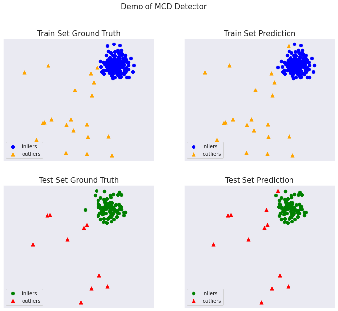
モデル訓練

pyod.models.mcd.MCD 検出器をインポートして初期化し、そしてモデルを適合させます。

最小共分散行列式 (MCD) を使用したガウス分布データセット内の外れ値を検出します : 共分散の堅牢な推定器です。

最小共分散行列式・共分散推定器はガウス分布データ上で適用されますが、単峰性の対称な分布からドローされたデータ上でも関連性がある可能性があります。それは多峰なデータで使用されることを意味していません (MinCovDet オブジェクトを適合させるために使用されるアルゴリズムはそのような場合には失敗する傾向にあります)。多峰なデータセットを処理するためには射影追跡法を考慮するべきです。

最初に最小共分散行列式モデルを適合させてからデータの外れ値の degree として Mahalanobis 距離を計算します。

参照 :

Johanna Hardin and David M Rocke. Outlier detection in the multiple cluster setting using the minimum covariance determinant estimator. Computational Statistics & Data Analysis, 44(4):625–638, 2004.
Peter J Rousseeuw and Katrien Van Driessen. A fast algorithm for the minimum covariance determinant estimator. Technometrics, 41(3):212–223, 1999.

from pyod.models.mcd import MCD

clf_name = 'MCD'
clf = MCD()
clf.fit(X_train)

MCD(assume_centered=False, contamination=0.1, random_state=None,
  store_precision=True, support_fraction=None)

訓練データの予測ラベルと外れ値スコアを取得します :

y_train_pred = clf.labels_  # binary labels (0: inliers, 1: outliers)
y_train_scores = clf.decision_scores_  # raw outlier scores

y_train_pred

array([0, 0, 0, 0, 0, 0, 0, 0, 0, 0, 0, 0, 0, 0, 0, 0, 0, 0, 0, 0, 0, 0,
       0, 0, 0, 0, 0, 0, 0, 0, 0, 0, 0, 0, 0, 0, 0, 0, 0, 0, 0, 0, 0, 0,
       0, 0, 0, 0, 0, 0, 0, 0, 0, 0, 1, 0, 0, 0, 0, 0, 0, 0, 0, 0, 0, 0,
       0, 0, 0, 0, 0, 0, 0, 0, 0, 0, 0, 0, 0, 0, 0, 0, 0, 0, 0, 0, 0, 0,
       0, 0, 0, 0, 0, 0, 0, 0, 0, 0, 0, 0, 0, 0, 0, 0, 0, 0, 0, 0, 0, 0,
       0, 0, 0, 0, 0, 0, 0, 0, 0, 0, 0, 0, 0, 0, 0, 0, 0, 0, 0, 0, 0, 0,
       0, 0, 0, 0, 0, 0, 0, 0, 0, 0, 0, 0, 0, 0, 0, 0, 0, 0, 0, 0, 0, 0,
       0, 0, 0, 0, 0, 0, 0, 0, 0, 0, 0, 0, 0, 0, 0, 0, 0, 0, 0, 0, 0, 0,
       0, 0, 0, 0, 1, 1, 1, 1, 1, 1, 1, 1, 1, 1, 0, 1, 1, 1, 1, 1, 1, 1,
       1, 1])

y_train_scores[-40:]

array([4.24565000e+00, 4.22664796e-01, 2.20854837e+00, 3.19271455e+00,
       5.28318116e+00, 4.89035191e+00, 9.00245383e+00, 3.36891011e+00,
       6.41160123e+00, 3.70486129e+00, 8.97553458e-01, 3.23785753e+00,
       3.55922222e-01, 6.19169925e+00, 7.27336532e-01, 3.88522610e+00,
       1.08105367e+00, 1.42204980e+01, 6.55858782e-01, 1.46394676e+00,
       3.95907542e+00, 1.06528255e-01, 6.75944610e-01, 4.94017438e+00,
       5.62629894e+00, 8.14443303e+00, 1.92662344e+00, 7.81555289e+00,
       1.17055228e-01, 6.62232486e-01, 9.36051952e+01, 1.76344612e+02,
       1.03037866e+02, 2.51116697e+02, 1.79382377e+01, 2.37451925e+01,
       1.80881699e+02, 1.72118668e+02, 1.27494937e+02, 6.26970512e+01])

予測と評価

先に正解ラベルを確認しておきます :

y_test

array([0., array([0., 0., 0., 0., 0., 0., 0., 0., 0., 0., 0., 0., 0., 0., 0., 0., 0.,
       0., 0., 0., 0., 0., 0., 0., 0., 0., 0., 0., 0., 0., 0., 0., 0., 0.,
       0., 0., 0., 0., 0., 0., 0., 0., 0., 0., 0., 0., 0., 0., 0., 0., 0.,
       0., 0., 0., 0., 0., 0., 0., 0., 0., 0., 0., 0., 0., 0., 0., 0., 0.,
       0., 0., 0., 0., 0., 0., 0., 0., 0., 0., 0., 0., 0., 0., 0., 0., 0.,
       0., 0., 0., 0., 0., 1., 1., 1., 1., 1., 1., 1., 1., 1., 1.])

テストデータ上で予測を行ないます :

y_test_pred = clf.predict(X_test)  # outlier labels (0 or 1)
y_test_scores = clf.decision_function(X_test)  # outlier scores

y_test_pred

array([0, 0, 0, 0, 0, 0, 0, 0, 0, 0, 0, 0, 0, 0, 0, 0, 0, 0, 0, 0, 0, 0,
       0, 1, 0, 0, 0, 0, 0, 0, 0, 0, 0, 0, 0, 0, 0, 0, 0, 0, 0, 0, 0, 0,
       0, 0, 0, 0, 0, 0, 0, 0, 0, 0, 0, 0, 0, 0, 0, 0, 0, 0, 0, 0, 0, 0,
       0, 0, 0, 0, 0, 0, 0, 0, 0, 0, 0, 1, 0, 0, 0, 0, 0, 0, 0, 0, 0, 0,
       0, 0, 1, 1, 1, 1, 1, 1, 1, 1, 1, 1])

y_test_scores[-40:]

array([ 5.9045124 , -2.01938422, -0.04809363,  1.579808  ,  7.29815783,
        2.75891915, 10.63424239,  1.69629951,  8.35181013,  3.87787154,
       -1.22952342,  2.30787057, -1.92598485,  8.78137251, -1.42671526,
        2.98254633, -1.05400309, 16.91238411, -1.38842923, -1.34779231,
        3.67815253, -1.95072358, -1.54857191,  3.38326885,  8.77706568,
       12.33489833, -0.87534863,  8.73047852, -1.9340466 , -1.4348534 ,
       26.06172492, 25.58479044, 25.93969245, 25.377791  , 22.11729834,
       23.73896701, 25.48826792, 26.29453172, 25.55043239, 25.38483225])

ROC と Precision @ Rank n pyod.utils.data.evaluate_print() を使用して予測を評価します。

from pyod.utils.data import evaluate_print
# evaluate and print the results
print("\nOn Training Data:")
evaluate_print(clf_name, y_train, y_train_scores)
print("\nOn Test Data:")
evaluate_print(clf_name, y_test, y_test_scores)

On Training Data:
MCD ROC:0.9986, precision @ rank n:0.95

On Test Data:
MCD ROC:1.0, precision @ rank n:1.0

総ての examples に含まれる visualize 関数により可視化を生成します :

from pyod.utils.example import visualize
 
visualize(clf_name, X_train, y_train, X_test, y_test, y_train_pred,
          y_test_pred, show_figure=True, save_figure=False)

以上

PyOD 0.8 : Examples : One Class SVM

06/27/2021

PyOD 0.8 : Examples : One Class SVM (解説)
翻訳 : (株)クラスキャットセールスインフォメーション
作成日時 : 06/27/2021 (0.8.9)

* 本ページは、PyOD の以下のドキュメントとサンプルを参考にして作成しています：

* ご自由にリンクを張って頂いてかまいませんが、sales-info@classcat.com までご一報いただけると嬉しいです。

★ 無料 Web セミナー開催中 ★ クラスキャット主催人工知能 & ビジネス Web セミナー

人工知能とビジネスをテーマに WEB セミナーを定期的に開催しています。
スケジュールは弊社公式 Web サイトでご確認頂けます。

お住まいの地域に関係なく Web ブラウザからご参加頂けます。事前登録 が必要ですのでご注意ください。
ウェビナー運用には弊社製品「ClassCat® Webinar」を利用しています。

クラスキャットは人工知能・テレワークに関する各種サービスを提供しております :

人工知能研究開発支援	人工知能研修サービス	テレワーク & オンライン授業を支援
PoC(概念実証)を失敗させないための支援 (本支援はセミナーに参加しアンケートに回答した方を対象としています。)

◆ お問合せ : 本件に関するお問い合わせ先は下記までお願いいたします。

株式会社クラスキャット セールス・マーケティング本部セールス・インフォメーション

E-Mail：sales-info@classcat.com ; WebSite: https://www.classcat.com/ ; Facebook

PyOD 0.8 : Examples : One Class SVM

完全なサンプル : examples/ocsvm_example.py

合成データの生成と可視化

pyod.utils.data.generate_data() でサンプルデータを生成します :

from pyod.utils.data import generate_data

contamination = 0.1  # percentage of outliers
n_train = 200  # number of training points
n_test = 100  # number of testing points

X_train, y_train, X_test, y_test = generate_data(
    n_train=n_train, n_test=n_test,
    n_features=2,
    contamination=contamination,
    random_state=42
)

X_train, y_train の shape と値を確認します :

print(X_train.shape)
print(y_train.shape)

(200, 2)
(200,)

X_train[:10]

array([[6.43365854, 5.5091683 ],
       [5.04469788, 7.70806466],
       [5.92453568, 5.25921966],
       [5.29399075, 5.67126197],
       [5.61509076, 6.1309285 ],
       [6.18590347, 6.09410578],
       [7.16630941, 7.22719133],
       [4.05470826, 6.48127032],
       [5.79978164, 5.86930893],
       [4.82256361, 7.18593123]])

y_train[:200]

array([0., 0., 0., 0., 0., 0., 0., 0., 0., 0., 0., 0., 0., 0., 0., 0., 0.,
       0., 0., 0., 0., 0., 0., 0., 0., 0., 0., 0., 0., 0., 0., 0., 0., 0.,
       0., 0., 0., 0., 0., 0., 0., 0., 0., 0., 0., 0., 0., 0., 0., 0., 0.,
       0., 0., 0., 0., 0., 0., 0., 0., 0., 0., 0., 0., 0., 0., 0., 0., 0.,
       0., 0., 0., 0., 0., 0., 0., 0., 0., 0., 0., 0., 0., 0., 0., 0., 0.,
       0., 0., 0., 0., 0., 0., 0., 0., 0., 0., 0., 0., 0., 0., 0., 0., 0.,
       0., 0., 0., 0., 0., 0., 0., 0., 0., 0., 0., 0., 0., 0., 0., 0., 0.,
       0., 0., 0., 0., 0., 0., 0., 0., 0., 0., 0., 0., 0., 0., 0., 0., 0.,
       0., 0., 0., 0., 0., 0., 0., 0., 0., 0., 0., 0., 0., 0., 0., 0., 0.,
       0., 0., 0., 0., 0., 0., 0., 0., 0., 0., 0., 0., 0., 0., 0., 0., 0.,
       0., 0., 0., 0., 0., 0., 0., 0., 0., 0., 1., 1., 1., 1., 1., 1., 1.,
       1., 1., 1., 1., 1., 1., 1., 1., 1., 1., 1., 1., 1.])

X_train の分布を可視化します :

import matplotlib.pyplot as plt
 
plt.scatter(X_train[:, 0], X_train[:, 1])

訓練データを可視化します :

import seaborn as sns
sns.set_style("dark")

from mpl_toolkits.mplot3d import Axes3D

X0 = X_train[:, 0]
X1 = X_train[:, 1]
Y = y_train

fig = plt.figure()
ax = Axes3D(fig)

ax.set_title("synthesized data")
 
ax.set_xlabel("X0")
ax.set_ylabel("X1")
ax.set_zlabel("Y")
 
ax.plot(X0, X1, Y, marker="o",linestyle='None')

モデル訓練

pyod.models.ocsvm.OCSVM 検出器をインポートして初期化し、そしてモデルを適合させます。

より多くの機能を持つ scikit-learn one-class SVM クラスのラッパーです。教師なし外れ値検知です。

高次元分布のサポートを推定します。実装は libsvm に基づいています。

参照 :

http://scikit-learn.org/stable/modules/svm.html#svm-outlier-detection
Bernhard Schölkopf, John C Platt, John Shawe-Taylor, Alex J Smola, and Robert C Williamson. Estimating the support of a high-dimensional distribution. Neural computation, 13(7):1443–1471, 2001.

パラメータ

kernel (string, optional (default=’rbf’)) :
アルゴリズムで使用されるカーネル・タイプを指定します。それは ‘linear’, ‘poly’, ‘rbf’, ‘sigmoid’, ‘precomputed’ の一つか callable でなければなりません。何も指定されない場合には、’rbf’ が使用されます。callable が与えられた場合にはカーネル行列を事前計算するために使用されます。

from pyod.models.ocsvm import OCSVM

clf_name = 'OneClassSVM'
clf = OCSVM()
clf.fit(X_train)

OCSVM(cache_size=200, coef0=0.0, contamination=0.1, degree=3, gamma='auto',
   kernel='rbf', max_iter=-1, nu=0.5, shrinking=True, tol=0.001,
   verbose=False)

訓練データの予測ラベルと外れ値スコアを得ます :

y_train_pred = clf.labels_  # binary labels (0: inliers, 1: outliers)
y_train_scores = clf.decision_scores_  # raw outlier scores

y_train_pred

array([0, 0, 0, 0, 0, 0, 0, 0, 0, 0, 0, 0, 0, 0, 0, 0, 0, 0, 0, 0, 0, 0,
       0, 0, 0, 0, 0, 0, 0, 0, 0, 0, 0, 0, 0, 0, 0, 0, 0, 0, 0, 0, 0, 0,
       0, 0, 0, 0, 0, 0, 0, 0, 0, 0, 1, 0, 0, 0, 0, 0, 0, 0, 0, 0, 0, 0,
       0, 0, 0, 0, 0, 0, 0, 0, 0, 0, 0, 0, 0, 0, 0, 0, 0, 0, 0, 0, 0, 0,
       0, 0, 0, 0, 0, 0, 0, 0, 0, 0, 0, 0, 0, 0, 0, 0, 0, 0, 0, 0, 0, 0,
       0, 0, 0, 0, 0, 0, 0, 0, 0, 0, 0, 0, 0, 0, 0, 0, 0, 0, 0, 0, 0, 0,
       0, 0, 0, 0, 0, 0, 0, 0, 0, 0, 0, 0, 0, 0, 0, 0, 0, 0, 0, 0, 0, 0,
       0, 0, 0, 0, 0, 0, 0, 0, 0, 0, 0, 0, 0, 0, 0, 0, 0, 0, 0, 0, 0, 0,
       0, 0, 0, 0, 1, 1, 1, 1, 1, 1, 1, 1, 1, 1, 0, 1, 1, 1, 1, 1, 1, 1,
       1, 1])

y_train_scores[-40:]

array([-0.78857197,  1.82421735,  0.52516778,  1.36053899, 15.95268822,
        2.4715799 , -1.98421762,  4.78992561, -1.49198395, -1.6983532 ,
        1.03366291,  3.6321792 , -2.00333481,  0.1132708 ,  1.1528244 ,
        1.47166268, -0.72974317, -1.55079259, -1.2506018 ,  1.15327899,
       23.92572607, 24.79414184, 24.02938483, 23.69938998, 25.22054002,
       22.76152076, 24.99977021, 23.81604268, 25.31886731, 24.14355787,
       13.71471089, 24.11178588, 25.36021672, 25.26198196, 25.20689073,
       25.25618027, 25.36017907, 24.76715117, 21.52711931, 25.30266924])

予測と評価

先に正解ラベルを確認しておきます :

y_test

array([0., array([0., 0., 0., 0., 0., 0., 0., 0., 0., 0., 0., 0., 0., 0., 0., 0., 0.,
       0., 0., 0., 0., 0., 0., 0., 0., 0., 0., 0., 0., 0., 0., 0., 0., 0.,
       0., 0., 0., 0., 0., 0., 0., 0., 0., 0., 0., 0., 0., 0., 0., 0., 0.,
       0., 0., 0., 0., 0., 0., 0., 0., 0., 0., 0., 0., 0., 0., 0., 0., 0.,
       0., 0., 0., 0., 0., 0., 0., 0., 0., 0., 0., 0., 0., 0., 0., 0., 0.,
       0., 0., 0., 0., 0., 1., 1., 1., 1., 1., 1., 1., 1., 1., 1.])

テストデータ上で予測を行ないます :

y_test_pred = clf.predict(X_test)  # outlier labels (0 or 1)
y_test_scores = clf.decision_function(X_test)  # outlier scores

y_test_pred

array([0, 0, 0, 0, 0, 0, 0, 0, 0, 0, 0, 0, 0, 0, 0, 0, 0, 0, 0, 0, 0, 0,
       0, 1, 0, 0, 0, 0, 0, 0, 0, 0, 0, 0, 0, 0, 0, 0, 0, 0, 0, 0, 0, 0,
       0, 0, 0, 0, 0, 0, 0, 0, 0, 0, 0, 0, 0, 0, 0, 0, 0, 0, 0, 0, 0, 0,
       0, 0, 0, 0, 0, 0, 0, 0, 0, 0, 0, 1, 0, 0, 0, 0, 0, 0, 0, 0, 0, 0,
       0, 0, 1, 1, 1, 1, 1, 1, 1, 1, 1, 1])

y_test_scores[-40:]

array([ 5.9045124 , -2.01938422, -0.04809363,  1.579808  ,  7.29815783,
        2.75891915, 10.63424239,  1.69629951,  8.35181013,  3.87787154,
       -1.22952342,  2.30787057, -1.92598485,  8.78137251, -1.42671526,
        2.98254633, -1.05400309, 16.91238411, -1.38842923, -1.34779231,
        3.67815253, -1.95072358, -1.54857191,  3.38326885,  8.77706568,
       12.33489833, -0.87534863,  8.73047852, -1.9340466 , -1.4348534 ,
       26.06172492, 25.58479044, 25.93969245, 25.377791  , 22.11729834,
       23.73896701, 25.48826792, 26.29453172, 25.55043239, 25.38483225])

ROC と Precision @ Rank n pyod.utils.data.evaluate_print() を使用して予測を評価します。

from pyod.utils.data import evaluate_print
# evaluate and print the results
print("\nOn Training Data:")
evaluate_print(clf_name, y_train, y_train_scores)
print("\nOn Test Data:")
evaluate_print(clf_name, y_test, y_test_scores)

On Training Data:
OneClassSVM ROC:0.9992, precision @ rank n:0.95

On Test Data:
OneClassSVM ROC:1.0, precision @ rank n:1.0

総ての examples に含まれる visualize 関数により可視化を生成します :

from pyod.utils.example import visualize
 
visualize(clf_name, X_train, y_train, X_test, y_test, y_train_pred,
          y_test_pred, show_figure=True, save_figure=False)

以上

PyOD 0.8 : Examples : 主成分分析 (PCA)

06/27/2021

PyOD 0.8 : Examples : 主成分分析 (PCA) (解説)
翻訳 : (株)クラスキャットセールスインフォメーション
作成日時 : 06/27/2021 (0.8.9)

* 本ページは、PyOD の以下のドキュメントとサンプルを参考にして作成しています：

* ご自由にリンクを張って頂いてかまいませんが、sales-info@classcat.com までご一報いただけると嬉しいです。

★ 無料 Web セミナー開催中 ★ クラスキャット主催人工知能 & ビジネス Web セミナー

人工知能とビジネスをテーマに WEB セミナーを定期的に開催しています。
スケジュールは弊社公式 Web サイトでご確認頂けます。

お住まいの地域に関係なく Web ブラウザからご参加頂けます。事前登録 が必要ですのでご注意ください。
ウェビナー運用には弊社製品「ClassCat® Webinar」を利用しています。

クラスキャットは人工知能・テレワークに関する各種サービスを提供しております :

人工知能研究開発支援	人工知能研修サービス	テレワーク & オンライン授業を支援
PoC(概念実証)を失敗させないための支援 (本支援はセミナーに参加しアンケートに回答した方を対象としています。)

◆ お問合せ : 本件に関するお問い合わせ先は下記までお願いいたします。

株式会社クラスキャット セールス・マーケティング本部セールス・インフォメーション

E-Mail：sales-info@classcat.com ; WebSite: https://www.classcat.com/ ; Facebook

PyOD 0.8 : Examples : 主成分分析 (PCA)

完全なサンプル : examples/pca_example.py

合成データの生成と可視化

pyod.utils.data.generate_data() でサンプルデータを生成します :

from pyod.utils.data import generate_data

contamination = 0.1  # percentage of outliers
n_train = 200  # number of training points
n_test = 100  # number of testing points

X_train, y_train, X_test, y_test = generate_data(
    n_train=n_train, n_test=n_test,
    contamination=contamination,
    random_state=42
)

※ ここでは特徴次元はデフォルトの 2 です。特徴次元 20 の場合についての試行は後述します。

X_train, y_train の shape と値を確認します :

print(X_train.shape)
print(y_train.shape)

(200, 2)
(200,)

X_train[:10]

array([[6.43365854, 5.5091683 ],
       [5.04469788, 7.70806466],
       [5.92453568, 5.25921966],
       [5.29399075, 5.67126197],
       [5.61509076, 6.1309285 ],
       [6.18590347, 6.09410578],
       [7.16630941, 7.22719133],
       [4.05470826, 6.48127032],
       [5.79978164, 5.86930893],
       [4.82256361, 7.18593123]])

y_train[:200]

array([0., 0., 0., 0., 0., 0., 0., 0., 0., 0., 0., 0., 0., 0., 0., 0., 0.,
       0., 0., 0., 0., 0., 0., 0., 0., 0., 0., 0., 0., 0., 0., 0., 0., 0.,
       0., 0., 0., 0., 0., 0., 0., 0., 0., 0., 0., 0., 0., 0., 0., 0., 0.,
       0., 0., 0., 0., 0., 0., 0., 0., 0., 0., 0., 0., 0., 0., 0., 0., 0.,
       0., 0., 0., 0., 0., 0., 0., 0., 0., 0., 0., 0., 0., 0., 0., 0., 0.,
       0., 0., 0., 0., 0., 0., 0., 0., 0., 0., 0., 0., 0., 0., 0., 0., 0.,
       0., 0., 0., 0., 0., 0., 0., 0., 0., 0., 0., 0., 0., 0., 0., 0., 0.,
       0., 0., 0., 0., 0., 0., 0., 0., 0., 0., 0., 0., 0., 0., 0., 0., 0.,
       0., 0., 0., 0., 0., 0., 0., 0., 0., 0., 0., 0., 0., 0., 0., 0., 0.,
       0., 0., 0., 0., 0., 0., 0., 0., 0., 0., 0., 0., 0., 0., 0., 0., 0.,
       0., 0., 0., 0., 0., 0., 0., 0., 0., 0., 1., 1., 1., 1., 1., 1., 1.,
       1., 1., 1., 1., 1., 1., 1., 1., 1., 1., 1., 1., 1.])

X_train の分布を可視化します :

import matplotlib.pyplot as plt
 
plt.scatter(X_train[:, 0], X_train[:, 1])

訓練データを可視化します :

import seaborn as sns
sns.set_style("dark")

from mpl_toolkits.mplot3d import Axes3D

X0 = X_train[:, 0]
X1 = X_train[:, 1]
Y = y_train

fig = plt.figure()
ax = Axes3D(fig)

ax.set_title("synthesized data")
 
ax.set_xlabel("X0")
ax.set_ylabel("X1")
ax.set_zlabel("Y")
 
ax.plot(X0, X1, Y, marker="o",linestyle='None')

モデル訓練

pyod.models.pca.PCA 検出器をインポートして初期化し、そしてモデルを適合させます。

主成分分析 (PCA) は外れ値の検出で利用できます。PCA はデータの特異値分解を使用してそれを低い次元空間に射影する線形次元削減です。

この手続きでは、データの共分散行列を固有値に関連する固有ベクトルと呼ばれる直交ベクトルに分解できます。高い固有値を持つ固有ベクトルはデータの殆どの分散を捕捉します。

従って、k 個の固有ベクトルから構成される低次元超平面はデータの殆どの分散を捕捉できます。けれども、外れ値は通常のデータポイントとは異なります、これは小さい固有値を持つ固有ベクトルにより構築される超平面上でより明瞭です。

従って、外れ値スコアは総ての固有ベクトル上のサンプルの射影された距離の合計として得られます。

参照 :

Charu C Aggarwal. Outlier analysis. In Data mining, 75–79. Springer, 2015.
Mei-Ling Shyu, Shu-Ching Chen, Kanoksri Sarinnapakorn, and LiWu Chang. A novel anomaly detection scheme based on principal component classifier. Technical Report, MIAMI UNIV CORAL GABLES FL DEPT OF ELECTRICAL AND COMPUTER ENGINEERING, 2003.

Score(X) = 選択された固有ベクトルにより構築された超平面への各サンプル間の加重ユークリッド距離の合計

パラメータ

n_components (int, float, None or string) :
保持するコンポーネント数。n_components が設定されない場合は総てのコンポーネントが保持されます :
```
n_components == min(n_samples, n_features)
```
if n_components == ‘mle’ and svd_solver == ‘full’, Minka’s MLE is used to guess the dimension if 0 < n_components < 1 and svd_solver == ‘full’, select the number of components such that the amount of variance that needs to be explained is greater than the percentage specified by n_components n_components cannot be equal to n_features for svd_solver == ‘arpack’.

from pyod.models.pca import PCA

# train PCA detector
clf_name = 'PCA'
clf = PCA(n_components=2)
clf.fit(X_train)

PCA(contamination=0.1, copy=True, iterated_power='auto', n_components=2,
  n_selected_components=None, random_state=None, standardization=True,
  svd_solver='auto', tol=0.0, weighted=True, whiten=False)

訓練データの予測ラベルと外れ値スコアを得ます :

y_train_pred = clf.labels_  # binary labels (0: inliers, 1: outliers)
y_train_scores = clf.decision_scores_  # raw outlier scores

y_train_pred

array([0, 0, 0, 0, 0, 0, 0, 0, 0, 0, 0, 0, 0, 0, 0, 0, 0, 0, 0, 0, 0, 0,
       0, 0, 0, 0, 1, 0, 0, 0, 0, 0, 0, 0, 0, 0, 0, 0, 0, 0, 0, 0, 1, 0,
       0, 0, 0, 0, 0, 0, 0, 0, 0, 0, 0, 0, 0, 0, 0, 0, 0, 0, 0, 0, 1, 0,
       0, 0, 0, 0, 0, 0, 0, 0, 0, 0, 0, 0, 0, 0, 0, 0, 0, 0, 0, 0, 0, 0,
       0, 0, 0, 0, 0, 0, 0, 0, 0, 0, 0, 1, 0, 0, 0, 0, 0, 0, 0, 0, 0, 0,
       0, 0, 0, 0, 0, 0, 0, 0, 0, 0, 0, 0, 0, 0, 0, 0, 0, 0, 0, 0, 0, 0,
       0, 0, 0, 0, 0, 0, 0, 0, 0, 0, 0, 0, 0, 0, 0, 0, 0, 0, 0, 0, 0, 0,
       0, 0, 0, 0, 0, 0, 0, 0, 0, 0, 0, 0, 0, 0, 0, 0, 0, 0, 0, 0, 0, 0,
       0, 0, 0, 0, 1, 1, 1, 1, 1, 0, 0, 1, 1, 1, 0, 1, 1, 1, 1, 1, 1, 1,
       0, 1])

y_train_scores[-40:]

array([ 9.4994967 ,  3.94506562,  9.70037971,  7.10016104,  8.3342693 ,
        5.20726666,  8.11879309,  7.09219081,  5.44404213,  8.13218023,
        4.1753126 , 11.30291142,  7.36028157,  6.47889712,  7.32111209,
        4.12430086,  9.53767094,  6.33863943,  7.44694126, 10.67688223,
       25.72127613, 26.62078588, 27.79438442, 30.53234151, 14.3121138 ,
        7.91069136, 12.34639345, 31.09120751, 34.48202163, 23.1528089 ,
        4.1915978 , 26.00171686, 30.43968531, 26.19059534, 32.35826934,
       37.28140553, 20.85589507, 22.29007341,  6.49340959, 32.82450057])

予測と評価

先に正解ラベルを確認しておきます :

y_test

array([0., array([0., 0., 0., 0., 0., 0., 0., 0., 0., 0., 0., 0., 0., 0., 0., 0., 0.,
       0., 0., 0., 0., 0., 0., 0., 0., 0., 0., 0., 0., 0., 0., 0., 0., 0.,
       0., 0., 0., 0., 0., 0., 0., 0., 0., 0., 0., 0., 0., 0., 0., 0., 0.,
       0., 0., 0., 0., 0., 0., 0., 0., 0., 0., 0., 0., 0., 0., 0., 0., 0.,
       0., 0., 0., 0., 0., 0., 0., 0., 0., 0., 0., 0., 0., 0., 0., 0., 0.,
       0., 0., 0., 0., 0., 1., 1., 1., 1., 1., 1., 1., 1., 1., 1.])

テストデータ上で予測を行ないます :

y_test_pred = clf.predict(X_test)  # outlier labels (0 or 1)
y_test_scores = clf.decision_function(X_test)  # outlier scores

y_test_pred

array([0, 0, 0, 0, 0, 0, 0, 0, 0, 0, 0, 0, 0, 0, 0, 0, 0, 0, 0, 0, 0, 0,
       0, 0, 0, 0, 0, 0, 0, 0, 0, 0, 0, 0, 0, 0, 0, 0, 0, 0, 1, 0, 0, 0,
       0, 0, 0, 0, 0, 0, 0, 0, 0, 0, 0, 0, 0, 0, 0, 0, 0, 0, 0, 0, 0, 0,
       1, 0, 0, 0, 0, 0, 0, 0, 0, 0, 0, 0, 0, 0, 0, 0, 0, 0, 0, 0, 0, 1,
       0, 0, 1, 1, 1, 1, 0, 0, 1, 1, 1, 1])

y_test_scores[-40:]

array([ 6.69788191,  8.10098946,  8.67589057,  4.03525639,  8.5173794 ,
       10.96951547, 13.39103421,  8.18804283, 10.88109875,  5.59854489,
        7.53977442,  8.51968901,  8.38421841,  8.98014699,  8.94552673,
       11.34805156,  8.33270878,  5.0861882 ,  6.08032842,  9.06872924,
       11.39917594,  6.67302445,  8.90946919, 10.3204397 ,  7.93996933,
       12.09701831,  9.18744095, 12.94755026,  6.66488304,  8.06232909,
       16.92393289, 28.21976824, 18.02857594, 33.10880243,  7.56515099,
        8.78663414, 28.21833459, 26.55191181, 24.05195145, 15.23121808])

ROC と Precision @ Rank n pyod.utils.data.evaluate_print() を使用して予測を評価します。

from pyod.utils.data import evaluate_print
# evaluate and print the results
print("\nOn Training Data:")
evaluate_print(clf_name, y_train, y_train_scores)
print("\nOn Test Data:")
evaluate_print(clf_name, y_test, y_test_scores)

On Training Data:
PCA ROC:0.8964, precision @ rank n:0.8

On Test Data:
PCA ROC:0.9033, precision @ rank n:0.8

総ての examples に含まれる visualize 関数により可視化を生成します :

from pyod.utils.example import visualize
 
visualize(clf_name, X_train, y_train, X_test, y_test, y_train_pred,
          y_test_pred, show_figure=True, save_figure=False)

特徴次元 20 の場合

from pyod.utils.data import generate_data

contamination = 0.1  # percentage of outliers
n_train = 200  # number of training points
n_test = 100  # number of testing points

X_train, y_train, X_test, y_test = generate_data(
    n_train=n_train, n_test=n_test,
    n_features=20,
    contamination=contamination,
    random_state=42
)

print(X_train.shape)
print(y_train.shape)

(200, 20)
(200,)

from pyod.models.pca import PCA

# train PCA detector
clf_name = 'PCA'
clf = PCA(n_components=3)
clf.fit(X_train)

PCA(contamination=0.1, copy=True, iterated_power='auto', n_components=3,
  n_selected_components=None, random_state=None, standardization=True,
  svd_solver='auto', tol=0.0, weighted=True, whiten=False)

y_train_pred = clf.labels_  # binary labels (0: inliers, 1: outliers)
y_train_scores = clf.decision_scores_  # raw outlier scores

y_test_pred = clf.predict(X_test)  # outlier labels (0 or 1)
y_test_scores = clf.decision_function(X_test)  # outlier scores

from pyod.utils.data import evaluate_print
# evaluate and print the results
print("\nOn Training Data:")
evaluate_print(clf_name, y_train, y_train_scores)
print("\nOn Test Data:")
evaluate_print(clf_name, y_test, y_test_scores)

On Training Data:
PCA ROC:1.0, precision @ rank n:1.0

On Test Data:
PCA ROC:1.0, precision @ rank n:1.0

以上

PyOD 0.8 : Examples : k 近傍法 & マハラノビス距離

06/26/2021

PyOD 0.8 : Examples : k 近傍法 & マハラノビス距離 (解説)
翻訳 : (株)クラスキャットセールスインフォメーション
作成日時 : 06/26/2021 (0.8.9)

* 本ページは、PyOD の以下のドキュメントとサンプルを参考にして作成しています：

* ご自由にリンクを張って頂いてかまいませんが、sales-info@classcat.com までご一報いただけると嬉しいです。

★ 無料 Web セミナー開催中 ★ クラスキャット主催人工知能 & ビジネス Web セミナー

人工知能とビジネスをテーマに WEB セミナーを定期的に開催しています。
スケジュールは弊社公式 Web サイトでご確認頂けます。

お住まいの地域に関係なく Web ブラウザからご参加頂けます。事前登録 が必要ですのでご注意ください。
ウェビナー運用には弊社製品「ClassCat® Webinar」を利用しています。

クラスキャットは人工知能・テレワークに関する各種サービスを提供しております :

人工知能研究開発支援	人工知能研修サービス	テレワーク & オンライン授業を支援
PoC(概念実証)を失敗させないための支援 (本支援はセミナーに参加しアンケートに回答した方を対象としています。)

◆ お問合せ : 本件に関するお問い合わせ先は下記までお願いいたします。

株式会社クラスキャット セールス・マーケティング本部セールス・インフォメーション

E-Mail：sales-info@classcat.com ; WebSite: https://www.classcat.com/ ; Facebook

PyOD 0.8 : Examples : k 近傍法 & マハラノビス距離

完全なサンプル : examples/knn_example.py

合成データの生成と可視化

pyod.utils.data.generate_data() でサンプルデータを生成します :

from pyod.utils.data import generate_data

contamination = 0.1  # percentage of outliers
n_train = 200  # number of training points
n_test = 100  # number of testing points

X_train, y_train, X_test, y_test = generate_data(
    n_train=n_train, n_test=n_test, contamination=contamination)

X_train, y_train の shape と値を確認します :

print(X_train.shape)
print(y_train.shape)

(200, 2)
(200,)

X_train[:10]

array([[3.08501648, 4.75998393],
       [4.13746077, 2.48731972],
       [3.79049305, 4.04812774],
       [3.96338469, 4.22143522],
       [4.2801191 , 3.74372575],
       [3.71259428, 3.50012167],
       [5.01925935, 3.85152323],
       [4.30397021, 4.26818773],
       [4.31568536, 3.33965944],
       [3.29025478, 4.32274734]])

y_train[:200]

array([0., 0., 0., 0., 0., 0., 0., 0., 0., 0., 0., 0., 0., 0., 0., 0., 0.,
       0., 0., 0., 0., 0., 0., 0., 0., 0., 0., 0., 0., 0., 0., 0., 0., 0.,
       0., 0., 0., 0., 0., 0., 0., 0., 0., 0., 0., 0., 0., 0., 0., 0., 0.,
       0., 0., 0., 0., 0., 0., 0., 0., 0., 0., 0., 0., 0., 0., 0., 0., 0.,
       0., 0., 0., 0., 0., 0., 0., 0., 0., 0., 0., 0., 0., 0., 0., 0., 0.,
       0., 0., 0., 0., 0., 0., 0., 0., 0., 0., 0., 0., 0., 0., 0., 0., 0.,
       0., 0., 0., 0., 0., 0., 0., 0., 0., 0., 0., 0., 0., 0., 0., 0., 0.,
       0., 0., 0., 0., 0., 0., 0., 0., 0., 0., 0., 0., 0., 0., 0., 0., 0.,
       0., 0., 0., 0., 0., 0., 0., 0., 0., 0., 0., 0., 0., 0., 0., 0., 0.,
       0., 0., 0., 0., 0., 0., 0., 0., 0., 0., 0., 0., 0., 0., 0., 0., 0.,
       0., 0., 0., 0., 0., 0., 0., 0., 0., 0., 1., 1., 1., 1., 1., 1., 1.,
       1., 1., 1., 1., 1., 1., 1., 1., 1., 1., 1., 1., 1.])

X_train の分布を可視化します :

import matplotlib.pyplot as plt
 
plt.scatter(X_train[:, 0], X_train[:, 1])

訓練データを可視化します :

import seaborn as sns
sns.set_style("dark")

from mpl_toolkits.mplot3d import Axes3D

X0 = X_train[:, 0]
X1 = X_train[:, 1]
Y = y_train

fig = plt.figure()
ax = Axes3D(fig)

ax.set_title("synthesized data")
 
ax.set_xlabel("X0")
ax.set_ylabel("X1")
ax.set_zlabel("Y")
 
ax.plot(X0, X1, Y, marker="o",linestyle='None')

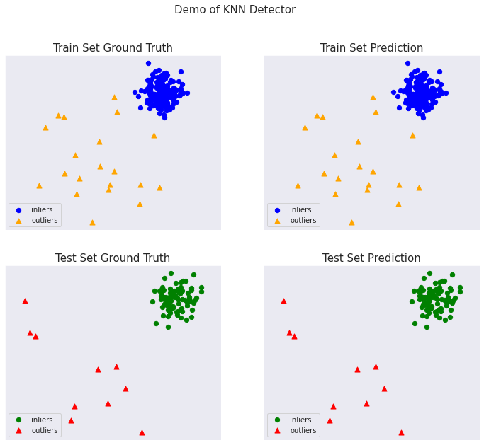
モデル訓練

pyod.models.knn.KNN 検出器をインポートして初期化し、そしてモデルを適合させます。

外れ値検知のための kNN クラス。観測について、その k-th 近傍への距離は外れ値スコアとして見なせるでしょう。それは密度を測定する方法としても見なせるでしょう。

参照 :

Fabrizio Angiulli and Clara Pizzuti. Fast outlier detection in high dimensional spaces. In European Conference on Principles of Data Mining and Knowledge Discovery, 15–27. Springer, 2002.
Sridhar Ramaswamy, Rajeev Rastogi, and Kyuseok Shim. Efficient algorithms for mining outliers from large data sets. In ACM Sigmod Record, volume 29, 427–438. ACM, 2000.

パラメータ

method (str, optional (default=’largest’)) – {‘largest’, ‘mean’, ‘median’}
- largest : k-th 近傍への距離を外れ値スコアとして使用します。
- mean : 総ての k 近傍への平均を外れ値スコアとして使用します。
- median : k 近傍への距離の中央値を外れ値スコアとして使用します。
algorithm ({‘auto’, ‘ball_tree’, ‘kd_tree’, ‘brute’}, optional) –
近傍を計算するために使用されるアルゴリズム :
- ’ball_tree’ は BallTree を使用します。
- ’kd_tree’ は KDTree を使用します。
- ’brute’ は brute-force 探索を使用します。
- ’auto’ は fit() メソッドに渡される値を基に最も適切なアルゴリズムを決定することを試みます。
Note: fitting on sparse input will override the setting of this parameter, using brute force.

Deprecated since version 0.74: algorithm is deprecated in PyOD 0.7.4 and will not be possible in 0.7.6. It has to use BallTree for consistency.
metric (string or callable, default ‘minkowski’) –
距離計算のために使用するメトリック。scikit-learn か scipy.spatial.distance からの任意のメトリックが使用できます。
metric_params (dict, optional (default = None)) –
metric 関数のための追加のキーワード引数。

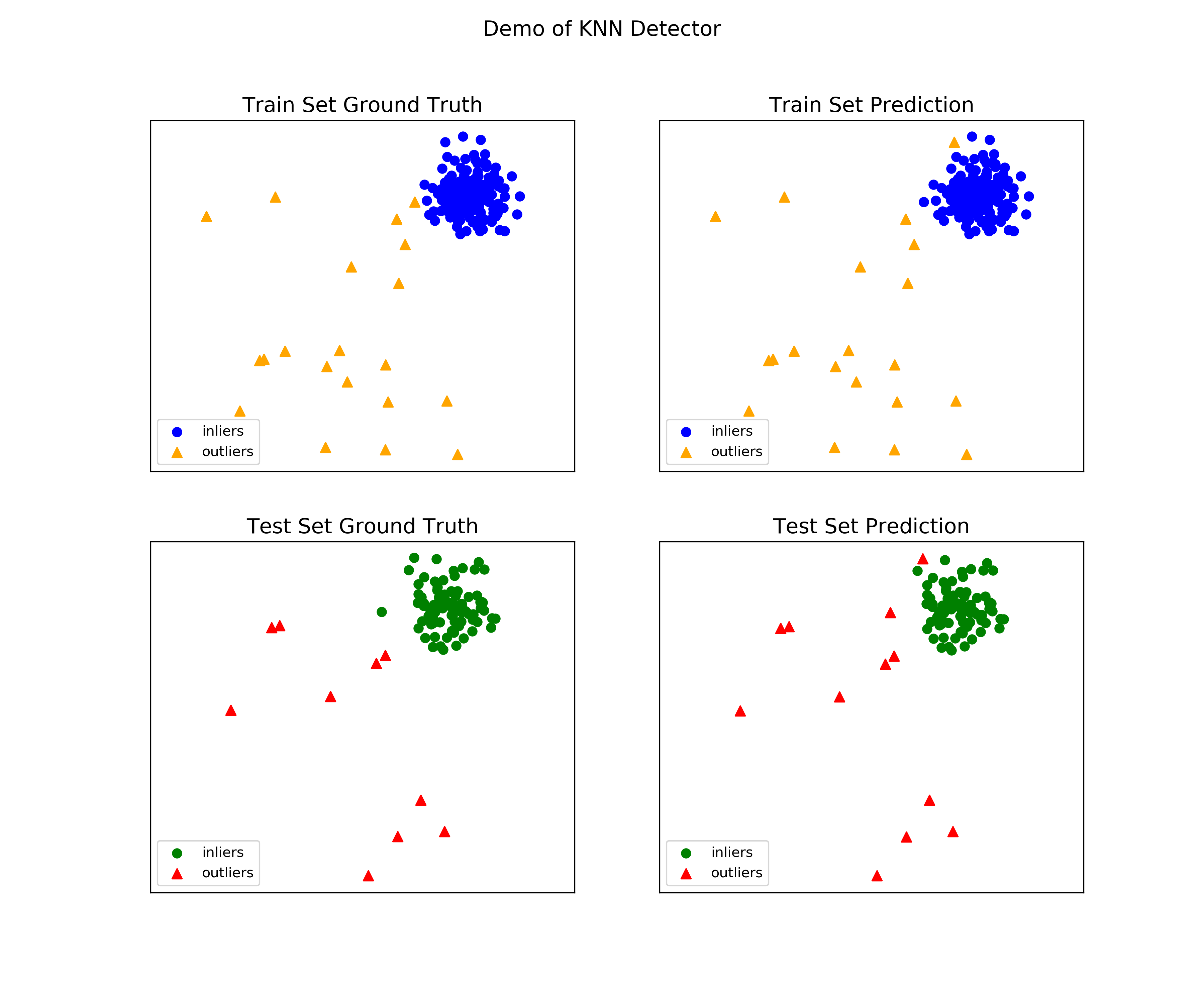
from pyod.models.knn import KNN   # kNN detector

# train kNN detector
clf_name = 'KNN'
clf = KNN()
clf.fit(X_train)

KNN(algorithm='auto', contamination=0.1, leaf_size=30, method='largest',
  metric='minkowski', metric_params=None, n_jobs=1, n_neighbors=5, p=2,
  radius=1.0)

訓練データの予測ラベルと外れ値スコアを得ます :

y_train_pred = clf.labels_  # binary labels (0: inliers, 1: outliers)
y_train_scores = clf.decision_scores_  # raw outlier scores

print(y_train_pred)

[0 0 0 0 0 0 0 0 0 0 0 0 0 0 0 0 0 0 0 0 0 0 0 0 0 0 0 0 0 0 0 0 0 0 0 0 0
 0 0 0 0 0 0 0 0 0 0 0 0 0 0 0 0 0 0 0 0 0 0 0 0 0 0 0 0 0 0 0 0 0 0 0 0 0
 0 0 0 0 0 0 0 0 0 0 0 0 0 0 0 0 0 0 0 0 0 0 0 0 0 0 0 0 0 0 0 0 0 0 0 0 0
 0 0 0 0 0 0 0 0 0 0 0 0 0 0 0 0 0 0 0 0 0 0 0 0 0 0 0 0 0 0 0 0 0 0 0 0 0
 0 0 0 0 0 0 0 0 0 0 0 0 0 0 0 0 0 0 0 0 0 0 0 0 0 0 0 0 0 0 0 0 1 1 1 1 1
 1 1 1 1 1 1 1 1 1 1 1 1 1 1 1]

y_train_scores[-40:]

[0.15962472 0.26404758 0.13328626 0.27473931 0.23961003 0.21293019
 0.1147517  0.49774753 0.197176   0.06412986 0.19258264 0.24692469
 0.1676141  0.25805756 0.1975197  0.13500727 0.2091096  0.18331466
 0.25338522 0.23136406 2.38800616 1.9625473  2.10956911 1.8785871
 2.50824404 1.9625473  1.88282016 3.259813   3.05440905 3.36664091
 1.65463831 2.00754852 3.53083084 3.53970455 1.50144057 1.72388028
 2.54678179 3.11133259 2.19112764 1.8785871 ]

予測と評価

正解ラベルを確認しておきます :

y_test

array([0., 0., 0., 0., 0., 0., 0., 0., 0., 0., 0., 0., 0., 0., 0., 0., 0.,
       0., 0., 0., 0., 0., 0., 0., 0., 0., 0., 0., 0., 0., 0., 0., 0., 0.,
       0., 0., 0., 0., 0., 0., 0., 0., 0., 0., 0., 0., 0., 0., 0., 0., 0.,
       0., 0., 0., 0., 0., 0., 0., 0., 0., 0., 0., 0., 0., 0., 0., 0., 0.,
       0., 0., 0., 0., 0., 0., 0., 0., 0., 0., 0., 0., 0., 0., 0., 0., 0.,
       0., 0., 0., 0., 0., 1., 1., 1., 1., 1., 1., 1., 1., 1., 1.])

テストデータ上の予測を行ないます :

y_test_pred = clf.predict(X_test)  # outlier labels (0 or 1)
y_test_scores = clf.decision_function(X_test)  # outlier scores

print(y_test.shape)
y_test_pred

(100,)
[0 0 0 0 0 0 0 0 0 0 0 0 0 0 0 0 0 0 0 0 0 0 0 0 0 0 0 0 0 0 0 0 0 0 0 0 0
 0 0 0 0 0 0 0 0 0 0 0 0 0 0 0 0 0 0 0 0 0 0 0 0 0 0 0 0 0 0 0 0 0 0 0 0 0
 0 0 0 0 0 0 0 0 0 0 0 0 0 0 0 0 1 1 1 1 1 1 1 1 1 1]

y_test_scores[-40:]

array([0.11599486, 0.1838938 , 0.22545484, 0.25303069, 0.19073255,
       0.16952675, 0.27454715, 0.12097446, 0.0909775 , 0.21331808,
       0.13385247, 0.25456906, 0.10869875, 0.13823526, 0.17606727,
       0.19224746, 0.16799589, 0.1532144 , 0.1298472 , 0.30639764,
       0.17532533, 0.22670677, 0.16088692, 0.36243913, 0.17956828,
       0.16300276, 0.08101652, 0.06396358, 0.15957843, 0.62192607,
       3.20652008, 1.97393657, 1.56580327, 1.81336178, 1.54919456,
       2.1308944 , 3.48636464, 2.24250892, 1.87019016, 4.78982494])

ROC と Precision @ Rank n pyod.utils.data.evaluate_print() を使用して予測を評価します。

from pyod.utils.data import evaluate_print
# evaluate and print the results
print("\nOn Training Data:")
evaluate_print(clf_name, y_train, y_train_scores)
print("\nOn Test Data:")
evaluate_print(clf_name, y_test, y_test_scores)

On Training Data:
KNN ROC:1.0, precision @ rank n:1.0

On Test Data:
KNN ROC:1.0, precision @ rank n:1.0

総ての examples に含まれる visualize 関数により可視化を生成します :

from pyod.utils.example import visualize
 
visualize(clf_name, X_train, y_train, X_test, y_test, y_train_pred,
          y_test_pred, show_figure=True, save_figure=False)

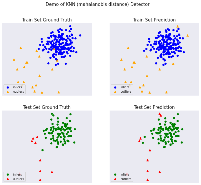
マハラノビス距離

完全なサンプル : examples/knn_mahalanobis_example.py

import numpy as np
from pyod.models.knn import KNN   # kNN detector

# mahalanobis 距離で kNN 検出器を訓練します。
clf_name = 'KNN (mahalanobis distance)'

# calculate covariance for mahalanobis distance
X_train_cov = np.cov(X_train, rowvar=False)
clf = KNN(algorithm='auto', metric='mahalanobis',
              metric_params={'V': X_train_cov})
clf.fit(X_train)

KNN(algorithm='auto', contamination=0.1, leaf_size=30, method='largest',
  metric='mahalanobis',
  metric_params={'V': array([[0.21822, 0.10856],
       [0.10856, 0.223  ]])},
  n_jobs=1, n_neighbors=5, p=2, radius=1.0)

訓練データの予測ラベルと外れ値スコアを得ます :

y_train_pred = clf.labels_  # binary labels (0: inliers, 1: outliers)
y_train_scores = clf.decision_scores_  # raw outlier scores

print(y_train_pred)

[0 0 0 0 0 0 0 0 0 0 0 0 0 1 0 0 0 0 0 0 0 0 0 0 0 0 0 0 0 0 0 0 0 0 0 0 0
 0 0 0 0 0 0 0 0 0 0 0 0 1 0 0 0 0 0 0 0 0 0 0 0 0 0 0 0 0 0 0 0 1 0 0 0 0
 0 0 0 0 0 0 0 0 0 0 0 0 0 0 0 0 0 0 0 0 0 0 0 0 0 0 0 0 0 0 0 0 0 0 0 0 0
 0 0 0 0 0 0 0 0 0 0 0 0 0 0 0 0 0 0 0 0 0 0 0 0 0 0 0 0 0 0 0 0 0 0 0 0 0
 0 0 0 0 0 0 0 0 0 0 0 0 0 0 0 0 0 0 0 0 0 0 0 0 0 0 0 0 0 0 0 0 1 1 1 1 1
 1 1 0 1 1 0 1 1 1 1 1 1 1 0 1]

y_train_scores[-40:]

array([0.58912848, 0.22380705, 0.27005879, 0.41356956, 0.23698991,
       0.26675444, 0.27765579, 0.24205096, 0.15355571, 0.27200349,
       0.26733088, 0.482192  , 0.33874355, 0.25996079, 0.24774249,
       0.1813697 , 0.1223033 , 0.27511716, 0.24852299, 0.20297293,
       1.55753928, 0.80804895, 0.75640102, 1.68413991, 1.63928778,
       1.52363689, 1.4012431 , 0.39888351, 1.36453714, 1.83193458,
       0.66176039, 1.1324612 , 1.33748243, 1.78087079, 1.07614616,
       1.3230474 , 1.37426469, 2.69424388, 0.22668787, 1.22162625])

正解ラベルを確認しておきます :

y_test

array([0., 0., 0., 0., 0., 0., 0., 0., 0., 0., 0., 0., 0., 0., 0., 0., 0.,
       0., 0., 0., 0., 0., 0., 0., 0., 0., 0., 0., 0., 0., 0., 0., 0., 0.,
       0., 0., 0., 0., 0., 0., 0., 0., 0., 0., 0., 0., 0., 0., 0., 0., 0.,
       0., 0., 0., 0., 0., 0., 0., 0., 0., 0., 0., 0., 0., 0., 0., 0., 0.,
       0., 0., 0., 0., 0., 0., 0., 0., 0., 0., 0., 0., 0., 0., 0., 0., 0.,
       0., 0., 0., 0., 0., 1., 1., 1., 1., 1., 1., 1., 1., 1., 1.])

テストデータ上の予測を行ないます :

y_test_pred = clf.predict(X_test)  # outlier labels (0 or 1)
y_test_scores = clf.decision_function(X_test)  # outlier scores

print(y_test.shape)
y_test_pred

(100,)
array([0, 0, 0, 0, 0, 0, 0, 0, 0, 0, 0, 0, 0, 0, 0, 1, 0, 0, 0, 0, 0, 0,
       0, 0, 0, 0, 0, 0, 0, 0, 0, 0, 0, 0, 1, 0, 0, 0, 0, 0, 0, 0, 0, 0,
       0, 0, 0, 0, 0, 0, 0, 0, 0, 0, 0, 0, 0, 0, 0, 0, 0, 0, 0, 0, 0, 0,
       0, 0, 0, 0, 0, 0, 0, 0, 0, 0, 0, 0, 0, 0, 1, 0, 0, 0, 0, 0, 0, 0,
       0, 0, 0, 1, 1, 1, 1, 1, 1, 0, 1, 1])

y_test_scores[-40:]

array([0.21432376, 0.33171001, 0.26295913, 0.18968928, 0.22568313,
       0.43079372, 0.43806264, 0.23698662, 0.56936528, 0.18924124,
       0.20143916, 0.13164876, 0.19035343, 0.28210869, 0.28090227,
       0.32447241, 0.27397147, 0.34668418, 0.29735364, 0.40047555,
       0.7764035 , 0.17145197, 0.38620828, 0.23455709, 0.17468498,
       0.20520947, 0.27625286, 0.18357644, 0.26571843, 0.20382472,
       0.73291695, 1.48326151, 1.04781778, 1.58587852, 1.25507347,
       1.65691819, 0.8926622 , 0.68944944, 1.6565503 , 0.96213366])

ROC と Precision @ Rank n pyod.utils.data.evaluate_print() を使用して予測を評価します。

from pyod.utils.data import evaluate_print
# evaluate and print the results
print("\nOn Training Data:")
evaluate_print(clf_name, y_train, y_train_scores)
print("\nOn Test Data:")
evaluate_print(clf_name, y_test, y_test_scores)

On Training Data:
KNN (mahalanobis distance) ROC:0.9594, precision @ rank n:0.85

On Test Data:
KNN (mahalanobis distance) ROC:0.9889, precision @ rank n:0.8

総ての examples に含まれる visualize 関数により可視化を生成します :

from pyod.utils.example import visualize
 
visualize(clf_name, X_train, y_train, X_test, y_test, y_train_pred,
          y_test_pred, show_figure=True, save_figure=False)

以上

PyOD 0.8 : 外れ値検知 101

06/26/2021

PyOD 0.8 : 外れ値検知 101 (翻訳/解説)
翻訳 : (株)クラスキャットセールスインフォメーション
作成日時 : 06/26/2021 (0.8.9)

* 本ページは、PyOD の以下のドキュメントの一部を翻訳した上で適宜、補足説明したものです：

Outlier Detection 101

* サンプルコードの動作確認はしておりますが、必要な場合には適宜、追加改変しています。
* ご自由にリンクを張って頂いてかまいませんが、sales-info@classcat.com までご一報いただけると嬉しいです。

★ 無料 Web セミナー開催中 ★ クラスキャット主催人工知能 & ビジネス Web セミナー

人工知能とビジネスをテーマに WEB セミナーを定期的に開催しています。
スケジュールは弊社公式 Web サイトでご確認頂けます。

お住まいの地域に関係なく Web ブラウザからご参加頂けます。事前登録 が必要ですのでご注意ください。
ウェビナー運用には弊社製品「ClassCat® Webinar」を利用しています。

クラスキャットは人工知能・テレワークに関する各種サービスを提供しております :

人工知能研究開発支援	人工知能研修サービス	テレワーク & オンライン授業を支援
PoC(概念実証)を失敗させないための支援 (本支援はセミナーに参加しアンケートに回答した方を対象としています。)

◆ お問合せ : 本件に関するお問い合わせ先は下記までお願いいたします。

株式会社クラスキャット セールス・マーケティング本部セールス・インフォメーション

E-Mail：sales-info@classcat.com ; WebSite: https://www.classcat.com/ ; Facebook

PyOD 0.8 : 外れ値検知 101

外れ値検知はサンプルの分布が与えられたとき異常であると考えられるかもしれない観測を識別するタスクとして広く参照されます。分布に属する任意の観測は inlier として参照され、任意の中心から離れた (= outlying) ポイントは外れ値として参照されます。

機械学習のコンテキストでは、このタスクのために 3 つの一般的なアプローチがあります :

1. 教師なし外れ値検知

(ラベル付けされていない) 訓練データは正常と異常な観測の両者を含みます。
モデルは fitting プロセスの間に外れ値を識別します。
このアプローチは、外れ値がデータの低密度領域に存在するポイントとして定義されるとき に取られます。
高密度領域に属さない任意の新しい観測は外れ値と考えられます。

2. 半教師あり Novelty (= 新規性) 検知

訓練データは正常な動作を記述する観測だけから成ります。
モデルは訓練データ上で fit されてから新しい観測を評価するために使用されます。
このアプローチは、外れ値が訓練データの分布とは異なるポイントとして定義されるとき に取られます。
閾値内の訓練データとは異なる任意の新しい観測は、それらが高密度領域を形成する場合でさえも、外れ値として考えられます。

3. 教師あり外れ値分類

総ての観測のための正解ラベル (inlier vs 外れ値) は既知です。
モデルは不均衡な訓練データ上で fit されてから新しい観測を分類するために使用されます。
このアプローチは正解が利用可能であるときに取られてそして外れ値が訓練セットと同じ分布に従うことを仮定しています。
任意の新しい観測はモデルを使用して分類されます。

PyOD で見つかるアルゴリズムは最初の 2 つのアプローチにフォーカスしています、これらは訓練データがどのように定義されるか、そしてモデル出力がどのように解釈されるかという点で異なります。更に学習することに関心があれば、関連する書籍、論文、動画とツールボックスのための Anomaly Detection Resources ページを参照してください。

以上

PyOD 0.8 : クイックスタート

06/25/2021

PyOD 0.8 : クイックスタート (翻訳/解説)
翻訳 : (株)クラスキャットセールスインフォメーション
作成日時 : 06/25/2021 (0.8.9)

* 本ページは、PyOD の以下のドキュメントの一部を翻訳した上で適宜、補足説明したものです：

★ 無料 Web セミナー開催中 ★ クラスキャット主催人工知能 & ビジネス Web セミナー

人工知能とビジネスをテーマに WEB セミナーを定期的に開催しています。
スケジュールは弊社公式 Web サイトでご確認頂けます。

お住まいの地域に関係なく Web ブラウザからご参加頂けます。事前登録 が必要ですのでご注意ください。
ウェビナー運用には弊社製品「ClassCat® Webinar」を利用しています。

クラスキャットは人工知能・テレワークに関する各種サービスを提供しております :

人工知能研究開発支援	人工知能研修サービス	テレワーク & オンライン授業を支援
PoC(概念実証)を失敗させないための支援 (本支援はセミナーに参加しアンケートに回答した方を対象としています。)

◆ お問合せ : 本件に関するお問い合わせ先は下記までお願いいたします。

株式会社クラスキャット セールス・マーケティング本部セールス・インフォメーション

E-Mail：sales-info@classcat.com ; WebSite: https://www.classcat.com/ ; Facebook

PyOD 0.8 : クイックスタート

機能チュートリアル

PyOD は幾つかの特集された投稿とチュートリアルにより機械学習コミュニティにより良く認知されています。

Analytics Vidhya : PyOD ライブラリを使用した Python で外れ値検知を学習する素晴らしいチュートリアル
KDnuggets : 外れ値検知法の直観的可視化, PyOD からの外れ値検知法の概要
Towards Data Science : ダミーのための異常検知
Computer Vision News (March 2019) : 外れ値検知のための Python オープンソース・ツールボックス
“examples/knn_example.py” は kNN 検出器を使用する基本的な API を実演します。総ての他のアルゴリズムに渡る API は一貫していて同様であることに注意してください。

外れ値検知のためのクイックスタート (kNN サンプル)

サンプルを実行するためのより詳細な手順は examples ディレクトリで見つけられます。

Full example: knn_example.py

モデルをインポートします。

from pyod.models.knn import KNN   # kNN detector

pyod.utils.data.generate_data() でサンプルデータを生成します :

contamination = 0.1  # percentage of outliers
n_train = 200  # number of training points
n_test = 100  # number of testing points

X_train, y_train, X_test, y_test = generate_data(
    n_train=n_train, n_test=n_test, contamination=contamination)

pyod.models.knn.KNN 検出器を初期化し、モデルを適合させ、そして予測を行ないます。

# train kNN detector
clf_name = 'KNN'
clf = KNN()
clf.fit(X_train)

# get the prediction labels and outlier scores of the training data
y_train_pred = clf.labels_  # binary labels (0: inliers, 1: outliers)
y_train_scores = clf.decision_scores_  # raw outlier scores

# get the prediction on the test data
y_test_pred = clf.predict(X_test)  # outlier labels (0 or 1)
y_test_scores = clf.decision_function(X_test)  # outlier scores

ROC と Precision @ Rank n (p@n) によって予測を評価します pyod.utils.data.evaluate_print()。

from pyod.utils.data import evaluate_print
# evaluate and print the results
print("\nOn Training Data:")
evaluate_print(clf_name, y_train, y_train_scores)
print("\nOn Test Data:")
evaluate_print(clf_name, y_test, y_test_scores)

訓練とテストデータの両者でサンプル出力を見ます。

On Training Data:
KNN ROC:1.0, precision @ rank n:1.0

On Test Data:
KNN ROC:0.9989, precision @ rank n:0.9

総てのサンプルに含まれる visualize 関数により可視化を生成します。

visualize(clf_name, X_train, y_train, X_test, y_test, y_train_pred,
          y_test_pred, show_figure=True, save_figure=False)

可視化 (knn_figure) :

様々なベース検出器からの外れ値スコアを組み合わせるためのクイックスタート

外れ値検知は教師なしの性質のためにしばしばモデルの不安定性に悩まされます。そのため、様々な検出器出力を組み合わせることが勧められます、例えば、その堅牢性を改良するために平均を取ることによって。検出器の組合せは外れ値アンサンブルの部分領域です ; より多くの情報については Aggarwal, C.C. and Sathe, S., 2017. Outlier ensembles: An introduction. Springer を参照してください。

4 つのスコアの組合せメカニズムがこのデモで示されます :

Average : 総ての検出器のスコアを平均する。
maximization : 総ての検出器に渡る最大スコア。
Average of Maximum (AOM) : ベース検出器をサブグループに分割して各サブグループの最大スコアを取ります。最終的なスコアは総てのサブグループのスコアの平均です。
Maximum of Average (MOA) : ベース検出器をサブグループに分割して各サブグループの平均スコアを取ります。最終的なスコアは総てのサブグループの最大値です。

“examples/comb_example.py” は複数のベース検出器の出力を組み合わせるための API を示します (comb_example.py, Jupyter Notebooks)。

Jupyter Noteboks については、”/notebooks/Model Combination.ipynb” をナビゲートしてください。

モデルをインポートしてサンプルデータを生成する。

from pyod.models.knn import KNN
from pyod.models.combination import aom, moa, average, maximization
from pyod.utils.data import generate_data

X, y = generate_data(train_only=True)  # load data

最初に異なる k (10 から 200) で 20kNN 外れ値検出器を初期化し、そして外れ値スコアを得ます。

# initialize 20 base detectors for combination
k_list = [10, 20, 30, 40, 50, 60, 70, 80, 90, 100, 110, 120, 130, 140,
            150, 160, 170, 180, 190, 200]

train_scores = np.zeros([X_train.shape[0], n_clf])
test_scores = np.zeros([X_test.shape[0], n_clf])

for i in range(n_clf):
    k = k_list[i]

    clf = KNN(n_neighbors=k, method='largest')
    clf.fit(X_train_norm)

    train_scores[:, i] = clf.decision_scores_
    test_scores[:, i] = clf.decision_function(X_test_norm)

次に出力スコアは組み合わせる前にゼロ平均と単位分散に標準化されます。このステップは検出器出力を同じスケールに調整するために重要です。
```
from pyod.utils.utility import standardizer

# scores have to be normalized before combination
train_scores_norm, test_scores_norm = standardizer(train_scores, test_scores)
```

そして上記のような 4 つの異なる組合せアルゴリズムが適用されます。

comb_by_average = average(test_scores_norm)
comb_by_maximization = maximization(test_scores_norm)
comb_by_aom = aom(test_scores_norm, 5) # 5 groups
comb_by_moa = moa(test_scores_norm, 5)) # 5 groups

最後に、総ての 4 つの組合せ方法が ROC と Precision @ Rank n で評価されます。

Combining 20 kNN detectors
Combination by Average ROC:0.9194, precision @ rank n:0.4531
Combination by Maximization ROC:0.9198, precision @ rank n:0.4688
Combination by AOM ROC:0.9257, precision @ rank n:0.4844
Combination by MOA ROC:0.9263, precision @ rank n:0.4688

以上

PyOD 0.8 : 概要

06/23/2021

PyOD 0.8 : 概要 (翻訳/解説)
翻訳 : (株)クラスキャットセールスインフォメーション
作成日時 : 06/25/2021 (0.8.9)

* 本ページは、PyOD の以下のドキュメントを翻訳した上で適宜、補足説明したものです：

★ 無料 Web セミナー開催中 ★ クラスキャット主催人工知能 & ビジネス Web セミナー

人工知能とビジネスをテーマに WEB セミナーを定期的に開催しています。
スケジュールは弊社公式 Web サイトでご確認頂けます。

お住まいの地域に関係なく Web ブラウザからご参加頂けます。事前登録 が必要ですのでご注意ください。
ウェビナー運用には弊社製品「ClassCat® Webinar」を利用しています。

クラスキャットは人工知能・テレワークに関する各種サービスを提供しております :

人工知能研究開発支援	人工知能研修サービス	テレワーク & オンライン授業を支援
PoC(概念実証)を失敗させないための支援 (本支援はセミナーに参加しアンケートに回答した方を対象としています。)

◆ お問合せ : 本件に関するお問い合わせ先は下記までお願いいたします。

株式会社クラスキャット セールス・マーケティング本部セールス・インフォメーション

E-Mail：sales-info@classcat.com ; WebSite: https://www.classcat.com/ ; Facebook

PyOD 0.8 : 概要

PyOD (Python Outlier Detection) は多変量データで中心を離れた (= outlying) オブジェクトを検知するための包括的でスケーラブルな Python ツールキットです。このエキサイティングなしかし挑戦的な分野は一般に外れ値検知 or 異常検知として言及されます。

PyOD は古典的 LOF (SIGMOD 2000) から最新の COPOD (ICDM 2020) まで、30 以上の検知アルゴリズムを含みます。2017 年から、PyOD [AZNL19] は数多くの学術的な研究と商用製品で成功的に利用されてきました [ AGSW19, ALCJ+19, AWDL+19, AZNHL19 ]。それはまた Analytics Vidhya, Towards Data Science, KDnuggets, Computer Vision News そして awesome-machine-learning を含む、様々な専門投稿/チュートリアルで機械学習コミュニティにより良く認知されています。

PyOD は以下のように特徴付けられます :

統一された API、詳細なドキュメント、そして様々なアルゴリズムに渡る対話的なサンプル。
高度なモデルは、scikit-learn からの古典的なもの、最新の深層学習メソッド、そして COPOD のような新しいアルゴリズムを含みます。
numba と joblib を使用し、可能なときには JIT と並列化による最適化されたパフォーマンス。
SUOD [ AZHC+21 ] による高速訓練 & 予測。
Python 2 & 3 の両者と互換。

API デモ :

# train the COPOD detector
from pyod.models.copod import COPOD
clf = COPOD()
clf.fit(X_train)

# get outlier scores
y_train_scores = clf.decision_scores_  # raw outlier scores
y_test_scores = clf.decision_function(X_test)  # outlier scores

Citing PyOD :

※ 原文を確認してください。

主要なリンクとリソース :

インストール

インストールのために pip を使用することが勧められます。最新バージョンがインストールされていることを確実にしてください、PyOD は頻繁にアップデートされるためです :

pip install pyod            # normal install
pip install --upgrade pyod  # or update if needed
pip install --pre pyod      # or include pre-release version for new features

代わりに、clone して setup.py ファイルを実行しても良いです :

git clone https://github.com/yzhao062/pyod.git
cd pyod
pip install .

必要な依存性 :

Python 2.7, 3.5, 3.6, or 3.7
combo>=0.0.8
joblib
numpy>=1.13
numba>=0.35
pandas>=0.25
scipy>=0.19.1
scikit_learn>=0.19.1
statsmodels

オプションの依存性 (詳細は下を見てください) :

combo (オプション, models/combination.py と FeatureBagging のために必要)
keras (オプション, AutoEncoder と他の深層学習モデルのために必要)
matplotlib (オプション, examples の実行のために必要)
pandas (オプション, benchmark の実行のために必要)
tensorflow (オプション, AutoEncoder と他の深層学習モデルのために必要)
xgboost (オプション, XGBOD のために必要)

警告 1 : PyOD は複数のニューラルネットワーク・ベースのモデルを持ちます、例えば AutoEncoder で、これは PyTorch と TensorFlow の両者で実装されています。けれども、PyOD は DL ライブラリを貴方のためにインストール しません。これは貴方のローカルコピーに干渉するリスクを軽減します。ニューラルネット・ベースのモデルを使用することを望む場合、Keras とバックエンド・ライブラリ、例えば TensorFlow がインストールされていることを確かにしてください。手順が提供されています : neural-net FAQ。同様に、XGBOD のような、xgboost に依存するモデルはデフォルトでは xgboost のインストールを強制 しません。

警告 2 : サンプルの実行は matplotlib を必要とします、これは mac OS 上の conda 仮想環境ではエラーを投げるかもしれません。理由と解法 mac_matplotlib を見てください。

警告 3 : PyOD は scikit-learn にも存在する複数のモデルを含みます。けれども、これら 2 つのライブラリの API は正確に同じではありません — 一貫性のためにそれらの一つだけを使用し、結果を混ぜないことを勧めます。より多くの情報については sckit-learn と PyOD の間の違いを参照してください。

API チートシート & リファレンス

完全な API リファレンス ( https://pyod.readthedocs.io/en/latest/pyod.html )。総ての検出器のための API チートシート :

fit(X) : 検出器を fit させます。
decision_function(X) : fit された検出器を使用して X の raw 異常スコアを予測します。
predict(X) : fit された検出器を使用して特定のサンプルが外れ値であるか否かを予測します。
predict_proba(X) : fit された検出器を使用してサンプルが外れ値である確率を予測します。

fit されたモデルの主要な属性 :

decision_scores_ : 訓練データの外れ値スコア。より高ければ、より異常です。外れ値は高いスコアを持つ傾向があります。
labels_ : 訓練データの二値ラベル。0 は inliers をそして 1 は外れ値/異常を表します。

Note : fit_predict() と fit_predict_score() は V0.6.9 では整合性のために deprecated となり、V0.8.0 で除去されます。To get the binary labels of the training data X_train, one should call clf.fit(X_train) and use clf.labels_, instead of calling clf.predict(X_train).

モデル・セーブ & ロード

PyOD はモデルの永続性に関して sklearn と同様のアプローチを取ります。明確にするため model persistence を見てください。

手短に言えば、PyOD モデルをセーブしてロードするために joblib や pickle を利用することを勧めます。例として “examples/save_load_model_example.py” を見てください。要するに、それは下のように単純です :

from joblib import dump, load

# save the model
dump(clf, 'clf.joblib')
# load the model
clf = load('clf.joblib')

実装アルゴリズム

PyOD ツールキットは 3 つの主要な機能グループから成ります :

(i) 個々の検知アルゴリズム :

PCA

線形モデル
主成分分析 (固有ベクトル超平面までの重み付けられた射影距離の合計)
2003
pyod.models.pca.PCA (クラス)
[ ASCSC03 ]

MCD

線形モデル
最小共分散行列式 (外れ値スコアとして mahalanobis を使用)
1999
pyod.models.mcd.MCD
[ AHR04, ARD99 ]

OCSVM

線形モデル
One-Class サポートベクターマシン
2001
pyod.models.ocsvm.OCSVM
[ AScholkopfPST+01 ]

MDD

線形モデル
偏差ベースの外れ値検知 (LMDD)
1996
pyod.models.lmdd.LMDD
[ AAAR96 ]

LOF

近接度ベース
局所外れ値因子 (= Local Outlier Factor)
2000
pyod.models.lof.LOF
[ ABKNS00 ]

COF

近接度ベース
接続性ベースの外れ値因子
2002
pyod.models.cof.COF
[ ATCFC02 ]

CBLOF

近接度ベース
クラスタリング・ベースの局所外れ値因子
2003
pyod.models.cblof.CBLOF
[ AHXD03 ]

LOCI

近接度ベース
LOCI: 局所相関積分を使用する高速外れ値検知
2003
pyod.models.loci.LOCI
[ APKGF03 ]

HBOS

近接度ベース
ヒストグラム・ベースの外れ値スコア
2012
pyod.models.hbos.HBOS
[ AGD12 ]

kNN

近接度ベース
k 近傍 (外れ値スコアとして kth 近傍への距離を使用)
2000
pyod.models.knn.KNN
[ AAP02, ARRS00 ]

AvgKNN

近接度ベース
平均 kNN (外れ値スコアとして k 近傍への平均距離を使用)
2002
pyod.models.knn.KNN
[ AAP02, ARRS00 ]

MedKNN

近接度ベース
中央値 kNN (外れ値スコアとして k 近傍への中央値距離を使用
2002
pyod.models.knn.KNN
[ AAP02, ARRS00 ]

SOD

近接度ベース
Subspace (部分空間) 外れ値検知
2009
pyod.models.sod.SOD
[ AKKrogerSZ09 ]

ROD

近接度ベース
Rotation ベースの外れ値検知
2020
pyod.models.rod.ROD
[ AABC20 ]

ABOD

確率的
Angle ベースの外れ値検知
2008
pyod.models.abod.ABOD
[ AKZ+08 ]

FastABOD

確率的
近似を使用する高速 Angle ベースの外れ値検知
2008
pyod.models.abod.ABOD
[ AKZ+08 ]

COPOD

確率的
COPOD: Copula-ベースの外れ値検知
2020
pyod.models.copod.COPOD
[ ALZB+20 ]

MAD

確率的
中央値絶対偏差 (MAD)
1993
pyod.models.mad.MAD
[ AIH93 ]

SOS

確率的
確率的外れ値選択
2012
pyod.models.sos.SOS
[ AJHuszarPvdH12 ]

IForest

外れ値アンサンブル
Isolation Forest
2008
pyod.models.iforest.IForest
[ ALTZ08, ALTZ12 ]

(短縮名なし)

外れ値アンサンブル
特徴バギング
2005
pyod.models.feature_bagging.FeatureBagging
[ ALK05 ]

LSCP

外れ値アンサンブル
LSCP: 並列外れ値アンサンブルの局所的選択的組み合わせ (Locally Selective Combination)
2019
pyod.models.lscp.LSCP
[ AZNHL19 ]

XGBOD

外れ値アンサンブル
Extreme Boosting ベースの外れ値検知 (教師あり)
2018
pyod.models.xgbod.XGBOD
[ AZH18 ]

LODA

外れ値アンサンブル
異常の軽量オンライン検出器
2016
pyod.models.loda.LODA
[ APevny16 ]

AutoEncoder

ニューラルネット
完全結合 AutoEncoder (外れ値スコアとして再構築エラーを使用)
2015
pyod.models.auto_encoder.AutoEncoder
[ AAgg15 ]

VAE

ニューラルネット
変分 AutoEncoder (外れ値スコアとして再構築エラーを使用)
2013
pyod.models.vae.VAE
[ AKW13 ]

Beta-VAE

ニューラルネット
変分 AutoEncoder (gamma and capacity を変化させることによる総てのカスタマイズされた損失項)
2018
pyod.models.vae.VAE
[ ABHP+18 ]

SO_GAAL

ニューラルネット
Single-Objective 敵対的生成 Active Learning
2019
pyod.models.so_gaal.SO_GAAL
[ ALLZ+19 ]

MO_GAAL

ニューラルネット
Multiple-Objective 敵対的生成 Active Learning
2019
pyod.models.mo_gaal.MO_GAAL
[ ALLZ+19 ]

(ii) 外れ値アンサンブル & 外れ値検出器 Combination フレームワーク :

(短縮名なし)

外れ値アンサンブル
特徴 Bagging
2005
pyod.models.feature_bagging.FeatureBagging
[ ALK05 ]

LSCP

外れ値アンサンブル
LSCP: 並列外れ値アンサンブルの局所的選択的組み合わせ (Locally Selective Combination)
2019
pyod.models.lscp.LSCP
[ AZNHL19 ]

XGBOD

外れ値アンサンブル
Extreme Boosting ベースの外れ値検知 (教師あり)
2018
pyod.models.xgbod.XGBOD
[ AZH18 ]

LODA

外れ値アンサンブル
異常の軽量オンライン検出器
2018
pyod.models.loda.LODA
[ APevny16 ]

Average

組合せ (= combination)
スコアの平均による単純な組合せ
2015
pyod.models.combination.average()
[ AAS15 ]

Weighted Average

組合せ
検出器重みを使用したスコアの平均による単純な組合せ
2015
pyod.models.combination.average()
[ AAS15 ]

Maximization

組合せ (= combination)
最大スコアを取ることによる単純な組合せ
2015
pyod.models.combination.maximization()
[ AAS15 ]

AOM

組合せ (= combination)
最大値の平均
2015
pyod.models.combination.aom()
[ AAS15 ]

MOA

組合せ (= combination)
平均値の最大化
2015
pyod.models.combination.moa()
[ AAS15 ]

Median

組合せ (= combination)
スコアの中央値を取ることによる単純な組合せ
2015
pyod.models.combination.median()
[ AAS15 ]

majority Vote

組合せ (= combination)
ラベルの投票の過半数を取ることによる単純な組合せ (重みが利用できます)
2015
pyod.models.combination.majority_vote()
[ AAS15 ]

(iii) ユティリティ関数 :

generate_data

データ
合成データ生成 ; 正規データは多変量ガウス分布により生成されそして外れ値は一様分布により生成されます。
pyod.utils.data.generate_data()
generate_data

generate_data_clusters

データ
クラスターの合成データ生成 ; より複雑なデータパターンが複数のクラスターで作成できます。
pyod.utils.data.generate_data_clusters()
generate_data_clusters

wpearsonr

統計
2 つのサンプルの重み付けられた Pearson 相関 (係数) を計算する
pyod.utils.stat_models.wpearsonr()
wpearsonr

get_label_n

ユティリティ
1 を top n 外れ値スコアに割り当てることにより raw 外れ値スコアを二値ラベルに変換します。
pyod.utils.utility.get_label_n()
get_label_n

precision_n_scores

ユティリティ
calculate precision @ rank n
pyod.utils.utility.precision_n_scores()
precision_n_scores

アルゴリズム・ベンチマーク

実装モデルの間の比較は下で利用可能です (図、compare_all_models.py、対話的な Jupyter Notebooks)。Jupyter Notebooks については、”/notebooks/Compare All Models.ipynb” をナビゲートしてください。

外れ値検知

ベンチマークはアルゴリズム選択のため実装されたモデルの概要を提供するために供給されます。トータルで、17 ベンチマーク・データセットが比較のために使用され、これは ODDS でダウンロードできます。

各データセットについて、それは最初に訓練のために 60% とテストのために 40% に分割されます。総ての実験はランダム分割で 10 回独立に繰り返されます。10 トライアルの平均が最終的な結果として見なされます。3 つの評価メトリクスが提供されます :

ROC (受信者操作特性) 曲線下の面積
精度 (= Precision) @ rank n (P@N)
実行時間

最新のベンチマークを確認してください。benchmark.py を実行することによりこのプロセスを再現できます。

リファレンス

AAgg15 : Charu C Aggarwal. Outlier analysis. In Data mining, 75–79. Springer, 2015.
AAS15(1,2,3,4,5,6,7) : Charu C Aggarwal and Saket Sathe. Theoretical foundations and algorithms for outlier ensembles. ACM SIGKDD Explorations Newsletter, 17(1):24–47, 2015.
AABC20 : Yahya Almardeny, Noureddine Boujnah, and Frances Cleary. A novel outlier detection method for multivariate data. IEEE Transactions on Knowledge and Data Engineering, 2020.
AAP02(1,2,3) : Fabrizio Angiulli and Clara Pizzuti. Fast outlier detection in high dimensional spaces. In European Conference on Principles of Data Mining and Knowledge Discovery, 15–27. Springer, 2002.
AAAR96 : Andreas Arning, Rakesh Agrawal, and Prabhakar Raghavan. A linear method for deviation detection in large databases. In KDD, volume 1141, 972–981. 1996.
ABKNS00 : Markus M Breunig, Hans-Peter Kriegel, Raymond T Ng, and Jörg Sander. Lof: identifying density-based local outliers. In ACM sigmod record, volume 29, 93–104. ACM, 2000.
ABHP+18 : Christopher P Burgess, Irina Higgins, Arka Pal, Loic Matthey, Nick Watters, Guillaume Desjardins, and Alexander Lerchner. Understanding disentangling in beta-vae. arXiv preprint arXiv:1804.03599, 2018.
AGD12 : Markus Goldstein and Andreas Dengel. Histogram-based outlier score (hbos): a fast unsupervised anomaly detection algorithm. KI-2012: Poster and Demo Track, pages 59–63, 2012.
AGSW19 : Parikshit Gopalan, Vatsal Sharan, and Udi Wieder. Pidforest: anomaly detection via partial identification. In Advances in Neural Information Processing Systems, 15783–15793. 2019.
AHR04 : Johanna Hardin and David M Rocke. Outlier detection in the multiple cluster setting using the minimum covariance determinant estimator. Computational Statistics & Data Analysis, 44(4):625–638, 2004.
AHXD03 : Zengyou He, Xiaofei Xu, and Shengchun Deng. Discovering cluster-based local outliers. Pattern Recognition Letters, 24(9-10):1641–1650, 2003.
AIH93 : Boris Iglewicz and David Caster Hoaglin. How to detect and handle outliers. Volume 16. Asq Press, 1993.
AJHuszarPvdH12 : JHM Janssens, Ferenc Huszár, EO Postma, and HJ van den Herik. Stochastic outlier selection. Technical Report, Technical report TiCC TR 2012-001, Tilburg University, Tilburg Center for Cognition and Communication, Tilburg, The Netherlands, 2012.
AKW13 : Diederik P Kingma and Max Welling. Auto-encoding variational bayes. arXiv preprint arXiv:1312.6114, 2013.
AKKrogerSZ09 : Hans-Peter Kriegel, Peer Kröger, Erich Schubert, and Arthur Zimek. Outlier detection in axis-parallel subspaces of high dimensional data. In Pacific-Asia Conference on Knowledge Discovery and Data Mining, 831–838. Springer, 2009.
AKZ+08(1,2) : Hans-Peter Kriegel, Arthur Zimek, and others. Angle-based outlier detection in high-dimensional data. In Proceedings of the 14th ACM SIGKDD international conference on Knowledge discovery and data mining, 444–452. ACM, 2008.
ALK05(1,2) : Aleksandar Lazarevic and Vipin Kumar. Feature bagging for outlier detection. In Proceedings of the eleventh ACM SIGKDD international conference on Knowledge discovery in data mining, 157–166. ACM, 2005.
ALCJ+19 : Dan Li, Dacheng Chen, Baihong Jin, Lei Shi, Jonathan Goh, and See-Kiong Ng. Mad-gan: multivariate anomaly detection for time series data with generative adversarial networks. In International Conference on Artificial Neural Networks, 703–716. Springer, 2019.
ALZB+20 : Zheng Li, Yue Zhao, Nicola Botta, Cezar Ionescu, and Xiyang Hu. COPOD: copula-based outlier detection. In IEEE International Conference on Data Mining (ICDM). IEEE, 2020.
ALTZ08 : Fei Tony Liu, Kai Ming Ting, and Zhi-Hua Zhou. Isolation forest. In Data Mining, 2008. ICDM’08. Eighth IEEE International Conference on, 413–422. IEEE, 2008.
ALTZ12 : Fei Tony Liu, Kai Ming Ting, and Zhi-Hua Zhou. Isolation-based anomaly detection. ACM Transactions on Knowledge Discovery from Data (TKDD), 6(1):3, 2012.
ALLZ+19(1,2) : Yezheng Liu, Zhe Li, Chong Zhou, Yuanchun Jiang, Jianshan Sun, Meng Wang, and Xiangnan He. Generative adversarial active learning for unsupervised outlier detection. IEEE Transactions on Knowledge and Data Engineering, 2019.
APKGF03 : Spiros Papadimitriou, Hiroyuki Kitagawa, Phillip B Gibbons, and Christos Faloutsos. Loci: fast outlier detection using the local correlation integral. In Data Engineering, 2003. Proceedings. 19th International Conference on, 315–326. IEEE, 2003.
APevny16(1,2) : Tomáš Pevn\`y. Loda: lightweight on-line detector of anomalies. Machine Learning, 102(2):275–304, 2016.
ARRS00(1,2,3) : Sridhar Ramaswamy, Rajeev Rastogi, and Kyuseok Shim. Efficient algorithms for mining outliers from large data sets. In ACM Sigmod Record, volume 29, 427–438. ACM, 2000.
ARD99 : Peter J Rousseeuw and Katrien Van Driessen. A fast algorithm for the minimum covariance determinant estimator. Technometrics, 41(3):212–223, 1999.
AScholkopfPST+01 : Bernhard Schölkopf, John C Platt, John Shawe-Taylor, Alex J Smola, and Robert C Williamson. Estimating the support of a high-dimensional distribution. Neural computation, 13(7):1443–1471, 2001.
ASCSC03 : Mei-Ling Shyu, Shu-Ching Chen, Kanoksri Sarinnapakorn, and LiWu Chang. A novel anomaly detection scheme based on principal component classifier. Technical Report, MIAMI UNIV CORAL GABLES FL DEPT OF ELECTRICAL AND COMPUTER ENGINEERING, 2003.
ATCFC02 : Jian Tang, Zhixiang Chen, Ada Wai-Chee Fu, and David W Cheung. Enhancing effectiveness of outlier detections for low density patterns. In Pacific-Asia Conference on Knowledge Discovery and Data Mining, 535–548. Springer, 2002.
AWDL+19 : Xuhong Wang, Ying Du, Shijie Lin, Ping Cui, Yuntian Shen, and Yupu Yang. Advae: a self-adversarial variational autoencoder with gaussian anomaly prior knowledge for anomaly detection. Knowledge-Based Systems, 2019.
AZH18(1,2) : Yue Zhao and Maciej K Hryniewicki. Xgbod: improving supervised outlier detection with unsupervised representation learning. In International Joint Conference on Neural Networks (IJCNN). IEEE, 2018.
AZHC+21 : Yue Zhao, Xiyang Hu, Cheng Cheng, Cong Wang, Changlin Wan, Wen Wang, Jianing Yang, Haoping Bai, Zheng Li, Cao Xiao, Yunlong Wang, Zhi Qiao, Jimeng Sun, and Leman Akoglu. Suod: accelerating large-scale unsupervised heterogeneous outlier detection. Proceedings of Machine Learning and Systems, 2021.
AZNHL19(1,2,3) : Yue Zhao, Zain Nasrullah, Maciej K Hryniewicki, and Zheng Li. LSCP: locally selective combination in parallel outlier ensembles. In Proceedings of the 2019 SIAM International Conference on Data Mining, SDM 2019, 585–593. Calgary, Canada, May 2019. SIAM.
URL: https://doi.org/10.1137/1.9781611975673.66, doi:10.1137/1.9781611975673.66.
AZNL19 : Yue Zhao, Zain Nasrullah, and Zheng Li. PyOD: a python toolbox for scalable outlier detection. Journal of Machine Learning Research, 20(96):1–7, 2019.

以上

タグアーカイブ: PyOD 0.8

PyOD 0.8 : Examples : AutoEncoder

合成データの生成

モデル訓練

予測と評価

PyOD 0.8 : Examples : Isolation Forest

合成データの生成と可視化

モデル訓練

予測と評価

PyOD 0.8 : Examples : 局所外れ値因子 (LOF)

合成データの生成と可視化

モデル訓練

予測と評価

PyOD 0.8 : Examples : 最小共分散行列式 (MCD)

合成データの生成と可視化

モデル訓練

予測と評価

PyOD 0.8 : Examples : One Class SVM

合成データの生成と可視化

モデル訓練

予測と評価

PyOD 0.8 : Examples : 主成分分析 (PCA)

合成データの生成と可視化

モデル訓練

予測と評価

特徴次元 20 の場合

PyOD 0.8 : Examples : k 近傍法 & マハラノビス距離

合成データの生成と可視化

モデル訓練

予測と評価

マハラノビス距離

PyOD 0.8 : 外れ値検知 101

1. 教師なし外れ値検知

2. 半教師あり Novelty (= 新規性) 検知

3. 教師あり外れ値分類

PyOD 0.8 : クイックスタート

機能チュートリアル

外れ値検知のためのクイックスタート (kNN サンプル)

様々なベース検出器からの外れ値スコアを組み合わせるためのクイックスタート

PyOD 0.8 : 概要

インストール

API チートシート & リファレンス

モデル・セーブ & ロード

実装アルゴリズム

アルゴリズム・ベンチマーク

リファレンス

ClassCat® Chatbot

人工知能開発支援

最近の投稿

カテゴリー

タグ