ホーム » 主成分分析
「主成分分析」カテゴリーアーカイブ
PyOD 0.8 : Examples : 主成分分析 (PCA)
PyOD 0.8 : Examples : 主成分分析 (PCA) (解説)
翻訳 : (株)クラスキャット セールスインフォメーション
作成日時 : 06/27/2021 (0.8.9)
* 本ページは、PyOD の以下のドキュメントとサンプルを参考にして作成しています:
* ご自由にリンクを張って頂いてかまいませんが、sales-info@classcat.com までご一報いただけると嬉しいです。

スケジュールは弊社 公式 Web サイト でご確認頂けます。
- お住まいの地域に関係なく Web ブラウザからご参加頂けます。事前登録 が必要ですのでご注意ください。
- ウェビナー運用には弊社製品「ClassCat® Webinar」を利用しています。
| 人工知能研究開発支援 | 人工知能研修サービス | テレワーク & オンライン授業を支援 |
| PoC(概念実証)を失敗させないための支援 (本支援はセミナーに参加しアンケートに回答した方を対象としています。) | ||
◆ お問合せ : 本件に関するお問い合わせ先は下記までお願いいたします。
| 株式会社クラスキャット セールス・マーケティング本部 セールス・インフォメーション |
| E-Mail:sales-info@classcat.com ; WebSite: https://www.classcat.com/ ; Facebook |

PyOD 0.8 : Examples : 主成分分析 (PCA)
完全なサンプル : examples/pca_example.py
合成データの生成と可視化
pyod.utils.data.generate_data() でサンプルデータを生成します :
from pyod.utils.data import generate_data

contamination = 0.1  # percentage of outliers
n_train = 200  # number of training points
n_test = 100  # number of testing points

X_train, y_train, X_test, y_test = generate_data(
    n_train=n_train, n_test=n_test,
    contamination=contamination,
    random_state=42
)
※ ここでは特徴次元はデフォルトの 2 です。特徴次元 20 の場合についての試行は後述します。
X_train, y_train の shape と値を確認します :
print(X_train.shape)
print(y_train.shape)
(200, 2)
(200,)
X_train[:10]
array([[6.43365854, 5.5091683 ],
       [5.04469788, 7.70806466],
       [5.92453568, 5.25921966],
       [5.29399075, 5.67126197],
       [5.61509076, 6.1309285 ],
       [6.18590347, 6.09410578],
       [7.16630941, 7.22719133],
       [4.05470826, 6.48127032],
       [5.79978164, 5.86930893],
       [4.82256361, 7.18593123]])
y_train[:200]
array([0., 0., 0., 0., 0., 0., 0., 0., 0., 0., 0., 0., 0., 0., 0., 0., 0.,
       0., 0., 0., 0., 0., 0., 0., 0., 0., 0., 0., 0., 0., 0., 0., 0., 0.,
       0., 0., 0., 0., 0., 0., 0., 0., 0., 0., 0., 0., 0., 0., 0., 0., 0.,
       0., 0., 0., 0., 0., 0., 0., 0., 0., 0., 0., 0., 0., 0., 0., 0., 0.,
       0., 0., 0., 0., 0., 0., 0., 0., 0., 0., 0., 0., 0., 0., 0., 0., 0.,
       0., 0., 0., 0., 0., 0., 0., 0., 0., 0., 0., 0., 0., 0., 0., 0., 0.,
       0., 0., 0., 0., 0., 0., 0., 0., 0., 0., 0., 0., 0., 0., 0., 0., 0.,
       0., 0., 0., 0., 0., 0., 0., 0., 0., 0., 0., 0., 0., 0., 0., 0., 0.,
       0., 0., 0., 0., 0., 0., 0., 0., 0., 0., 0., 0., 0., 0., 0., 0., 0.,
       0., 0., 0., 0., 0., 0., 0., 0., 0., 0., 0., 0., 0., 0., 0., 0., 0.,
       0., 0., 0., 0., 0., 0., 0., 0., 0., 0., 1., 1., 1., 1., 1., 1., 1.,
       1., 1., 1., 1., 1., 1., 1., 1., 1., 1., 1., 1., 1.])
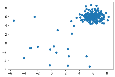
X_train の分布を可視化します :
import matplotlib.pyplot as plt

plt.scatter(X_train[:, 0], X_train[:, 1])
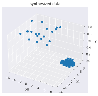
訓練データを可視化します :
import seaborn as sns
sns.set_style("dark")

from mpl_toolkits.mplot3d import Axes3D

X0 = X_train[:, 0]
X1 = X_train[:, 1]
Y = y_train

fig = plt.figure()
ax = Axes3D(fig)

ax.set_title("synthesized data")

ax.set_xlabel("X0")
ax.set_ylabel("X1")
ax.set_zlabel("Y")

ax.plot(X0, X1, Y, marker="o",linestyle='None')
モデル訓練
pyod.models.pca.PCA 検出器をインポートして初期化し、そしてモデルを適合させます。
主成分分析 (PCA) は外れ値の検出で利用できます。PCA はデータの特異値分解を使用してそれを低い次元空間に射影する線形次元削減です。
この手続きでは、データの共分散行列を固有値に関連する固有ベクトルと呼ばれる直交ベクトルに分解できます。高い固有値を持つ固有ベクトルはデータの殆どの分散を捕捉します。
従って、k 個の固有ベクトルから構成される低次元超平面はデータの殆どの分散を捕捉できます。けれども、外れ値は通常のデータポイントとは異なります、これは小さい固有値を持つ固有ベクトルにより構築される超平面上でより明瞭です。
従って、外れ値スコアは総ての固有ベクトル上のサンプルの射影された距離の合計として得られます。
参照 :
- Charu C Aggarwal. Outlier analysis. In Data mining, 75–79. Springer, 2015.
- Mei-Ling Shyu, Shu-Ching Chen, Kanoksri Sarinnapakorn, and LiWu Chang. A novel anomaly detection scheme based on principal component classifier. Technical Report, MIAMI UNIV CORAL GABLES FL DEPT OF ELECTRICAL AND COMPUTER ENGINEERING, 2003.
Score(X) = 選択された固有ベクトルにより構築された超平面への各サンプル間の加重ユークリッド距離の合計
パラメータ
- n_components (int, float, None or string) :
保持するコンポーネント数。n_components が設定されない場合は総てのコンポーネントが保持されます :n_components == min(n_samples, n_features)if n_components == ‘mle’ and svd_solver == ‘full’, Minka’s MLE is used to guess the dimension if 0 < n_components < 1 and svd_solver == ‘full’, select the number of components such that the amount of variance that needs to be explained is greater than the percentage specified by n_components n_components cannot be equal to n_features for svd_solver == ‘arpack’.
from pyod.models.pca import PCA

# train PCA detector
clf_name = 'PCA'
clf = PCA(n_components=2)
clf.fit(X_train)
PCA(contamination=0.1, copy=True, iterated_power='auto', n_components=2,
  n_selected_components=None, random_state=None, standardization=True,
  svd_solver='auto', tol=0.0, weighted=True, whiten=False)
訓練データの予測ラベルと外れ値スコアを得ます :
y_train_pred = clf.labels_  # binary labels (0: inliers, 1: outliers)
y_train_scores = clf.decision_scores_  # raw outlier scores
y_train_pred
array([0, 0, 0, 0, 0, 0, 0, 0, 0, 0, 0, 0, 0, 0, 0, 0, 0, 0, 0, 0, 0, 0,
       0, 0, 0, 0, 1, 0, 0, 0, 0, 0, 0, 0, 0, 0, 0, 0, 0, 0, 0, 0, 1, 0,
       0, 0, 0, 0, 0, 0, 0, 0, 0, 0, 0, 0, 0, 0, 0, 0, 0, 0, 0, 0, 1, 0,
       0, 0, 0, 0, 0, 0, 0, 0, 0, 0, 0, 0, 0, 0, 0, 0, 0, 0, 0, 0, 0, 0,
       0, 0, 0, 0, 0, 0, 0, 0, 0, 0, 0, 1, 0, 0, 0, 0, 0, 0, 0, 0, 0, 0,
       0, 0, 0, 0, 0, 0, 0, 0, 0, 0, 0, 0, 0, 0, 0, 0, 0, 0, 0, 0, 0, 0,
       0, 0, 0, 0, 0, 0, 0, 0, 0, 0, 0, 0, 0, 0, 0, 0, 0, 0, 0, 0, 0, 0,
       0, 0, 0, 0, 0, 0, 0, 0, 0, 0, 0, 0, 0, 0, 0, 0, 0, 0, 0, 0, 0, 0,
       0, 0, 0, 0, 1, 1, 1, 1, 1, 0, 0, 1, 1, 1, 0, 1, 1, 1, 1, 1, 1, 1,
       0, 1])
y_train_scores[-40:]
array([ 9.4994967 ,  3.94506562,  9.70037971,  7.10016104,  8.3342693 ,
        5.20726666,  8.11879309,  7.09219081,  5.44404213,  8.13218023,
        4.1753126 , 11.30291142,  7.36028157,  6.47889712,  7.32111209,
        4.12430086,  9.53767094,  6.33863943,  7.44694126, 10.67688223,
       25.72127613, 26.62078588, 27.79438442, 30.53234151, 14.3121138 ,
        7.91069136, 12.34639345, 31.09120751, 34.48202163, 23.1528089 ,
        4.1915978 , 26.00171686, 30.43968531, 26.19059534, 32.35826934,
       37.28140553, 20.85589507, 22.29007341,  6.49340959, 32.82450057])
予測と評価
先に正解ラベルを確認しておきます :
y_test
array([0., array([0., 0., 0., 0., 0., 0., 0., 0., 0., 0., 0., 0., 0., 0., 0., 0., 0.,
       0., 0., 0., 0., 0., 0., 0., 0., 0., 0., 0., 0., 0., 0., 0., 0., 0.,
       0., 0., 0., 0., 0., 0., 0., 0., 0., 0., 0., 0., 0., 0., 0., 0., 0.,
       0., 0., 0., 0., 0., 0., 0., 0., 0., 0., 0., 0., 0., 0., 0., 0., 0.,
       0., 0., 0., 0., 0., 0., 0., 0., 0., 0., 0., 0., 0., 0., 0., 0., 0.,
       0., 0., 0., 0., 0., 1., 1., 1., 1., 1., 1., 1., 1., 1., 1.])
テストデータ上で予測を行ないます :
y_test_pred = clf.predict(X_test)  # outlier labels (0 or 1)
y_test_scores = clf.decision_function(X_test)  # outlier scores
y_test_pred
array([0, 0, 0, 0, 0, 0, 0, 0, 0, 0, 0, 0, 0, 0, 0, 0, 0, 0, 0, 0, 0, 0,
       0, 0, 0, 0, 0, 0, 0, 0, 0, 0, 0, 0, 0, 0, 0, 0, 0, 0, 1, 0, 0, 0,
       0, 0, 0, 0, 0, 0, 0, 0, 0, 0, 0, 0, 0, 0, 0, 0, 0, 0, 0, 0, 0, 0,
       1, 0, 0, 0, 0, 0, 0, 0, 0, 0, 0, 0, 0, 0, 0, 0, 0, 0, 0, 0, 0, 1,
       0, 0, 1, 1, 1, 1, 0, 0, 1, 1, 1, 1])
y_test_scores[-40:]
array([ 6.69788191,  8.10098946,  8.67589057,  4.03525639,  8.5173794 ,
       10.96951547, 13.39103421,  8.18804283, 10.88109875,  5.59854489,
        7.53977442,  8.51968901,  8.38421841,  8.98014699,  8.94552673,
       11.34805156,  8.33270878,  5.0861882 ,  6.08032842,  9.06872924,
       11.39917594,  6.67302445,  8.90946919, 10.3204397 ,  7.93996933,
       12.09701831,  9.18744095, 12.94755026,  6.66488304,  8.06232909,
       16.92393289, 28.21976824, 18.02857594, 33.10880243,  7.56515099,
        8.78663414, 28.21833459, 26.55191181, 24.05195145, 15.23121808])
ROC と Precision @ Rank n pyod.utils.data.evaluate_print() を使用して予測を評価します。
from pyod.utils.data import evaluate_print
# evaluate and print the results
print("\nOn Training Data:")
evaluate_print(clf_name, y_train, y_train_scores)
print("\nOn Test Data:")
evaluate_print(clf_name, y_test, y_test_scores)
On Training Data:
PCA ROC:0.8964, precision @ rank n:0.8

On Test Data:
PCA ROC:0.9033, precision @ rank n:0.8
総ての examples に含まれる visualize 関数により可視化を生成します :
from pyod.utils.example import visualize

visualize(clf_name, X_train, y_train, X_test, y_test, y_train_pred,
          y_test_pred, show_figure=True, save_figure=False)
特徴次元 20 の場合
from pyod.utils.data import generate_data

contamination = 0.1  # percentage of outliers
n_train = 200  # number of training points
n_test = 100  # number of testing points

X_train, y_train, X_test, y_test = generate_data(
    n_train=n_train, n_test=n_test,
    n_features=20,
    contamination=contamination,
    random_state=42
)
print(X_train.shape)
print(y_train.shape)
(200, 20)
(200,)
from pyod.models.pca import PCA

# train PCA detector
clf_name = 'PCA'
clf = PCA(n_components=3)
clf.fit(X_train)
PCA(contamination=0.1, copy=True, iterated_power='auto', n_components=3,
  n_selected_components=None, random_state=None, standardization=True,
  svd_solver='auto', tol=0.0, weighted=True, whiten=False)
y_train_pred = clf.labels_  # binary labels (0: inliers, 1: outliers)
y_train_scores = clf.decision_scores_  # raw outlier scores
y_test_pred = clf.predict(X_test)  # outlier labels (0 or 1)
y_test_scores = clf.decision_function(X_test)  # outlier scores
from pyod.utils.data import evaluate_print
# evaluate and print the results
print("\nOn Training Data:")
evaluate_print(clf_name, y_train, y_train_scores)
print("\nOn Test Data:")
evaluate_print(clf_name, y_test, y_test_scores)
On Training Data:
PCA ROC:1.0, precision @ rank n:1.0

On Test Data:
PCA ROC:1.0, precision @ rank n:1.0
以上
ClassCat® Chatbot
人工知能開発支援
- テクニカルコンサルティングサービス
- 実証実験 (プロトタイプ構築)
- アプリケーションへの実装
- 人工知能研修サービス
クラスキャット
セールス・インフォメーション
E-Mail:sales-info@classcat.com