ホーム » 外れ値検知
「外れ値検知」カテゴリーアーカイブ
Prophet 1.0 : 外れ値
Prophet 1.0 : 外れ値 (翻訳/解説)
翻訳 : (株)クラスキャット セールスインフォメーション
作成日時 : 07/13/2021 (1.0)
* 本ページは、Prophet の以下のドキュメントを翻訳した上で適宜、補足説明したものです:
* サンプルコードの動作確認はしておりますが、必要な場合には適宜、追加改変しています。
* ご自由にリンクを張って頂いてかまいませんが、sales-info@classcat.com までご一報いただけると嬉しいです。

スケジュールは弊社 公式 Web サイト でご確認頂けます。
- お住まいの地域に関係なく Web ブラウザからご参加頂けます。事前登録 が必要ですのでご注意ください。
- ウェビナー運用には弊社製品「ClassCat® Webinar」を利用しています。
| 人工知能研究開発支援 | 人工知能研修サービス | テレワーク & オンライン授業を支援 |
| PoC(概念実証)を失敗させないための支援 (本支援はセミナーに参加しアンケートに回答した方を対象としています。) | ||
◆ お問合せ : 本件に関するお問い合わせ先は下記までお願いいたします。
| 株式会社クラスキャット セールス・マーケティング本部 セールス・インフォメーション |
| E-Mail:sales-info@classcat.com ; WebSite: https://www.classcat.com/ ; Facebook |
Prophet 1.0 : 外れ値
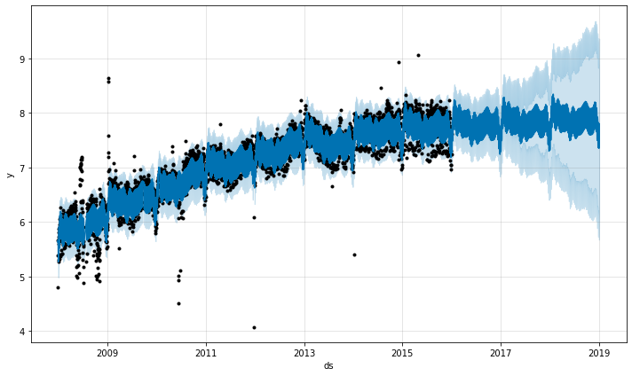
外れ値が Prophet の予測に影響を与えられる 2 つの主要な方法があります。ここでは前からの R ページへのログ記録された Wikipedia アクセスの予測を行ないますが、不良データのブロックを伴います。
df = pd.read_csv('../examples/example_wp_log_R_outliers1.csv')
m = Prophet()
m.fit(df)
future = m.make_future_dataframe(periods=1096)
forecast = m.predict(future)
fig = m.plot(forecast)
トレンド予測は合理的に見えますが、不確定区間は広すぎるようです。Prophet は履歴の外れ値を処理できますが、トレンド変化でそれらを適合させることによってのみです。そして不確実性モデルは同様の大きさの未来のトレンド変化を想定します。
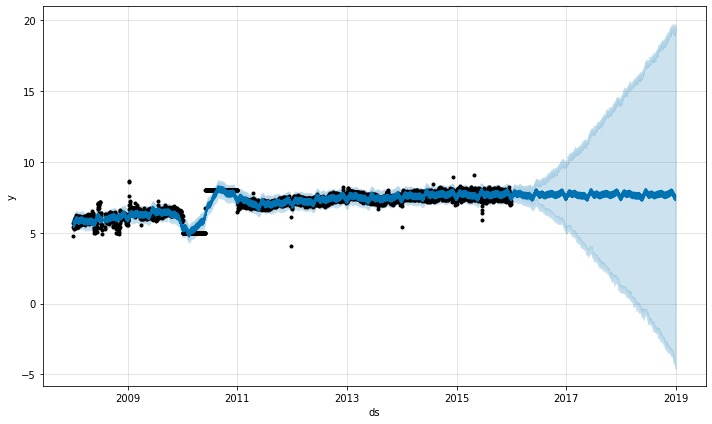
外れ値を扱う最善の方法はそれらを除去することです – Prophet はデータが欠落しても問題ありません。履歴でそれらの値を NA に設定してしかし未来の日付はそのままにする場合、Prophet はそれらの値の予測を与えます。
df.loc[(df['ds'] > '2010-01-01') & (df['ds'] < '2011-01-01'), 'y'] = None
model = Prophet().fit(df)
fig = model.plot(model.predict(future))

上の例では外れ値は不確実性推定を台無しにしましたが主要な予測 yhat には影響を与えませんでした。追加された外れ値をもつこの例でのように、これは常には当てはまりません :
df = pd.read_csv('../examples/example_wp_log_R_outliers2.csv')
m = Prophet()
m.fit(df)
future = m.make_future_dataframe(periods=1096)
forecast = m.predict(future)
fig = m.plot(forecast)
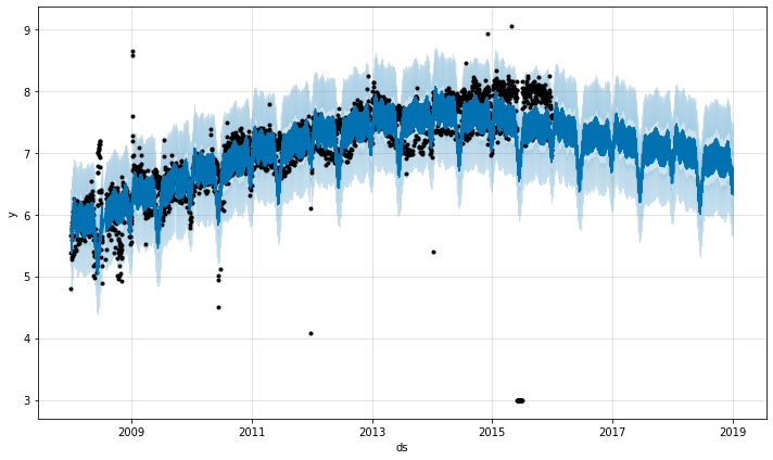
ここでは 2015年6月の極端な外れ値は季節性推定を台無しにしていますので、それらの効果は未来に永遠に響きます。再度、正しいアプローチはそれらを除去することです :
df.loc[(df['ds'] > '2015-06-01') & (df['ds'] < '2015-06-30'), 'y'] = None
m = Prophet().fit(df)
fig = m.plot(m.predict(future))
以上
Alibi Detect 0.7 : Examples : 外れ値、敵対的 & ドリフト検知 on CIFAR10
Alibi Detect 0.7 : Examples : 外れ値、敵対的 & ドリフト検知 on CIFAR10 (翻訳/解説)
翻訳 : (株)クラスキャット セールスインフォメーション
作成日時 : 07/04/2021 (0.7.0)
* 本ページは、Alibi Detect の以下のドキュメントを翻訳した上で適宜、補足説明したものです:
* サンプルコードの動作確認はしておりますが、必要な場合には適宜、追加改変しています。
* ご自由にリンクを張って頂いてかまいませんが、sales-info@classcat.com までご一報いただけると嬉しいです。
スケジュールは弊社 公式 Web サイト でご確認頂けます。
- お住まいの地域に関係なく Web ブラウザからご参加頂けます。事前登録 が必要ですのでご注意ください。
- ウェビナー運用には弊社製品「ClassCat® Webinar」を利用しています。
| 人工知能研究開発支援 | 人工知能研修サービス | テレワーク & オンライン授業を支援 |
| PoC(概念実証)を失敗させないための支援 (本支援はセミナーに参加しアンケートに回答した方を対象としています。) | ||
◆ お問合せ : 本件に関するお問い合わせ先は下記までお願いいたします。
| 株式会社クラスキャット セールス・マーケティング本部 セールス・インフォメーション |
| E-Mail:sales-info@classcat.com ; WebSite: https://www.classcat.com/ ; Facebook |
Alibi Detect 0.7 : Examples : 外れ値、敵対的 & ドリフト検知 on CIFAR10
0. データセット
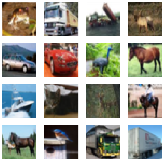
CIFAR10 は 10 クラス : 飛行機、自動車、鳥、猫、鹿、犬、カエル、馬、船とトラック – に渡り均等に分配された 60,000 の 32 x 32 RGB 画像から成ります。
# imports and plot examples
import matplotlib.pyplot as plt
%matplotlib inline
import tensorflow as tf

(X_train, y_train), (X_test, y_test) = tf.keras.datasets.cifar10.load_data()
X_train = X_train.astype('float32') / 255
X_test = X_test.astype('float32') / 255
y_train = y_train.astype('int64').reshape(-1,)
y_test = y_test.astype('int64').reshape(-1,)
print('Train: ', X_train.shape, y_train.shape)
print('Test: ', X_test.shape, y_test.shape)

plt.figure(figsize=(10, 10))
n = 4
for i in range(n ** 2):
    plt.subplot(n, n, i + 1)
    plt.imshow(X_train[i])
    plt.axis('off')
plt.show();
Train:  (50000, 32, 32, 3) (50000,)
Test:  (10000, 32, 32, 3) (10000,)
1. 変分オートエンコーダ (VAE) による外れ値検知
メソッド
簡単に言えば :
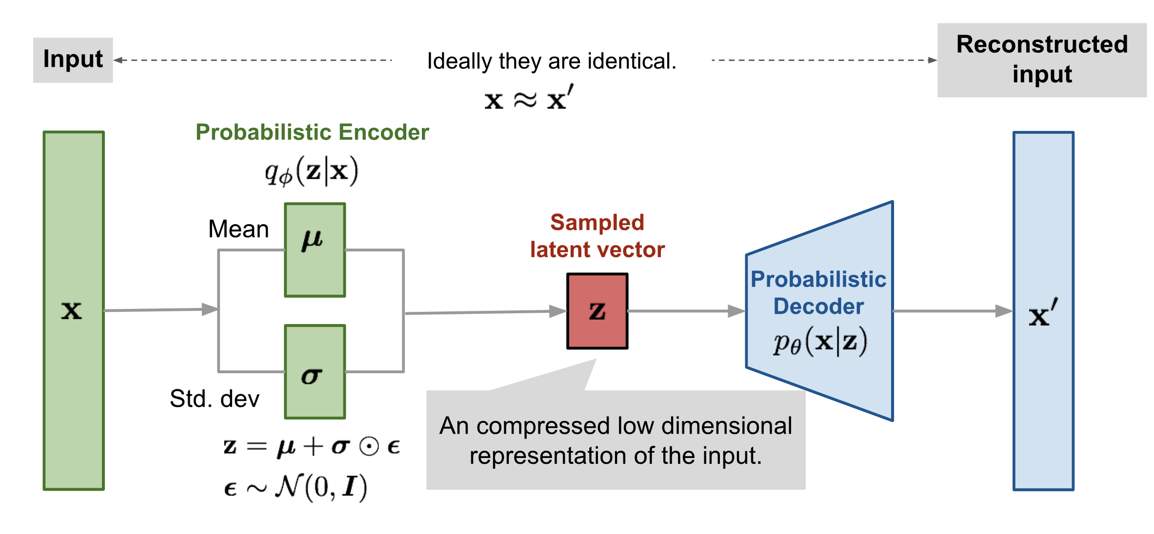
- 正常データ上で VAE を訓練するのでそれは inlier を上手く再構築できます。
- VAE が incoming リクエストを上手く再構築できないのであれば?外れ値です!
画像ソース: https://lilianweng.github.io/lil-log/2018/08/12/from-autoencoder-to-beta-vae.html
# more imports
import logging
import numpy as np
import os

from tensorflow.keras.layers import Conv2D, Conv2DTranspose, Dense
from tensorflow.keras.layers import Flatten, Layer, Reshape, InputLayer
from tensorflow.keras.regularizers import l1

from alibi_detect.od import OutlierVAE
from alibi_detect.utils.fetching import fetch_detector
from alibi_detect.utils.perturbation import apply_mask
from alibi_detect.utils.saving import save_detector, load_detector
from alibi_detect.utils.visualize import plot_instance_score, plot_feature_outlier_image

logger = tf.get_logger()
logger.setLevel(logging.ERROR)
検知器をロードまたはスクラッチから訓練する
ノートブックで使用される事前訓練済みの外れ値と敵対的検知器は ここ で見つかります。組込みの fetch_detector 関数を利用できます、これは事前訓練モデルをローカルディレクトリ filepath にセーブして検知器をロードします。代わりに、スクラッチから検知器を訓練することができます :
load_pretrained = False
%%time
filepath = os.path.join(os.getcwd(), 'outlier')

if load_pretrained:  # load pre-trained detector
    detector_type = 'outlier'
    dataset = 'cifar10'
    detector_name = 'OutlierVAE'
    od = fetch_detector(filepath, detector_type, dataset, detector_name)
    filepath = os.path.join(filepath, detector_name)
else:  # define model, initialize, train and save outlier detector

    # define encoder and decoder networks
    latent_dim = 1024
    encoder_net = tf.keras.Sequential(
      [
          InputLayer(input_shape=(32, 32, 3)),
          Conv2D(64, 4, strides=2, padding='same', activation=tf.nn.relu),
          Conv2D(128, 4, strides=2, padding='same', activation=tf.nn.relu),
          Conv2D(512, 4, strides=2, padding='same', activation=tf.nn.relu)
      ]
    )

    decoder_net = tf.keras.Sequential(
      [
          InputLayer(input_shape=(latent_dim,)),
          Dense(4*4*128),
          Reshape(target_shape=(4, 4, 128)),
          Conv2DTranspose(256, 4, strides=2, padding='same', activation=tf.nn.relu),
          Conv2DTranspose(64, 4, strides=2, padding='same', activation=tf.nn.relu),
          Conv2DTranspose(3, 4, strides=2, padding='same', activation='sigmoid')
      ]
    )

    # initialize outlier detector
    od = OutlierVAE(
        threshold=.015,  # threshold for outlier score
        encoder_net=encoder_net,  # can also pass VAE model instead
        decoder_net=decoder_net,  # of separate encoder and decoder
        latent_dim=latent_dim
    )

    # train
    od.fit(X_train, epochs=50, verbose=True)

    # save the trained outlier detector
    save_detector(od, filepath)
782/782 [=] - 32s 36ms/step - loss: 3328.0921
782/782 [=] - 29s 36ms/step - loss: -2477.8159
782/782 [=] - 29s 36ms/step - loss: -3505.9077
782/782 [=] - 29s 36ms/step - loss: -4018.4684
782/782 [=] - 29s 36ms/step - loss: -4339.1812
782/782 [=] - 29s 36ms/step - loss: -4564.4784
782/782 [=] - 29s 36ms/step - loss: -4752.0325
782/782 [=] - 29s 36ms/step - loss: -4909.1439
782/782 [=] - 29s 36ms/step - loss: -5027.7148
782/782 [=] - 29s 36ms/step - loss: -5108.3359
782/782 [=] - 29s 36ms/step - loss: -5183.5322
782/782 [=] - 29s 36ms/step - loss: -5221.8213
782/782 [=] - 29s 36ms/step - loss: -5286.5078
782/782 [=] - 29s 36ms/step - loss: -5336.4698
782/782 [=] - 29s 36ms/step - loss: -5390.1145
782/782 [=] - 29s 36ms/step - loss: -5435.4759
782/782 [=] - 29s 36ms/step - loss: -5469.5508
782/782 [=] - 29s 36ms/step - loss: -5513.7060
782/782 [=] - 29s 36ms/step - loss: -5546.3630
782/782 [=] - 29s 36ms/step - loss: -5586.9172
782/782 [=] - 29s 36ms/step - loss: -5604.6617
782/782 [=] - 29s 36ms/step - loss: -5638.2204
782/782 [=] - 29s 36ms/step - loss: -5657.4971
782/782 [=] - 29s 36ms/step - loss: -5684.9612
782/782 [=] - 29s 36ms/step - loss: -5706.7390
782/782 [=] - 29s 36ms/step - loss: -5719.2535
782/782 [=] - 29s 36ms/step - loss: -5742.7461
782/782 [=] - 29s 36ms/step - loss: -5760.9044
782/782 [=] - 29s 36ms/step - loss: -5777.8526
782/782 [=] - 29s 36ms/step - loss: -5793.0808
782/782 [=] - 29s 36ms/step - loss: -5803.5456
782/782 [=] - 29s 36ms/step - loss: -5822.1962
782/782 [=] - 29s 36ms/step - loss: -5821.3968
782/782 [=] - 29s 36ms/step - loss: -5847.5206
782/782 [=] - 29s 36ms/step - loss: -5855.4035
782/782 [=] - 29s 36ms/step - loss: -5866.9793
782/782 [=] - 29s 36ms/step - loss: -5879.4730
782/782 [=] - 29s 36ms/step - loss: -5885.7166
782/782 [=] - 29s 36ms/step - loss: -5895.9667
782/782 [=] - 29s 36ms/step - loss: -5905.9128
782/782 [=] - 29s 36ms/step - loss: -5913.2937
782/782 [=] - 29s 36ms/step - loss: -5922.4864
782/782 [=] - 29s 36ms/step - loss: -5930.4101
782/782 [=] - 29s 36ms/step - loss: -5935.5514
782/782 [=] - 29s 36ms/step - loss: -5942.9960
782/782 [=] - 29s 36ms/step - loss: -5953.9588
782/782 [=] - 29s 36ms/step - loss: -5959.2278
782/782 [=] - 29s 36ms/step - loss: -5962.3586
782/782 [=] - 29s 36ms/step - loss: -5967.2992
782/782 [=] - 29s 36ms/step - loss: -5975.1563
Directory /home/ubuntu/ws.alibi_detect/outlier does not exist and is now created.
CPU times: user 24min 6s, sys: 22.3 s, total: 24min 28s
Wall time: 24min 8s
モデルが in-distribution 訓練データを何とか再構築できるかを確認しましょう :
# plot original and reconstructed instance
idx = 8
X = X_train[idx].reshape(1, 32, 32, 3)
X_recon = od.vae(X)
plt.imshow(X.reshape(32, 32, 3)); plt.axis('off'); plt.show()
plt.imshow(X_recon.numpy().reshape(32, 32, 3)); plt.axis('off'); plt.show()


閾値を設定する
良い閾値を見つけることは技巧的であり得ます、何故ならばそれらは典型的には解釈することが容易でないからです。infer_threshold メソッドは sensible な値を見つけるのに役立ちます。インスタンスのバッチ X を渡してそれらの何パーセントを正常であると考えるかを threshold_perc を通して指定する必要があります。
print('Current threshold: {}'.format(od.threshold))
od.infer_threshold(X_train, threshold_perc=99, batch_size=128)  # assume 1% of the training data are outliers
print('New threshold: {}'.format(od.threshold))
Current threshold: 0.015
New threshold: 0.00969364859163762
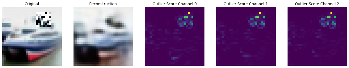
外れ値を作成して検知する
元のインスタンスにランダムノイズマスクを適用することにより幾つかの外れ値を作成できます :
np.random.seed(0)

i = 1

# create masked instance
x = X_test[i].reshape(1, 32, 32, 3)
x_mask, mask = apply_mask(
    x,
    mask_size=(8,8),
    n_masks=1,
    channels=[0,1,2],
    mask_type='normal',
    noise_distr=(0,1),
    clip_rng=(0,1)
)

# predict outliers and reconstructions
sample = np.concatenate([x_mask, x])
preds = od.predict(sample)
x_recon = od.vae(sample).numpy()
# check if outlier and visualize outlier scores
labels = ['No!', 'Yes!']
print(f"Is original outlier? {labels[preds['data']['is_outlier'][1]]}")
print(f"Is perturbed outlier? {labels[preds['data']['is_outlier'][0]]}")
plot_feature_outlier_image(preds, sample, x_recon, max_instances=1)
Is original outlier? No!
Is perturbed outlier? Yes!
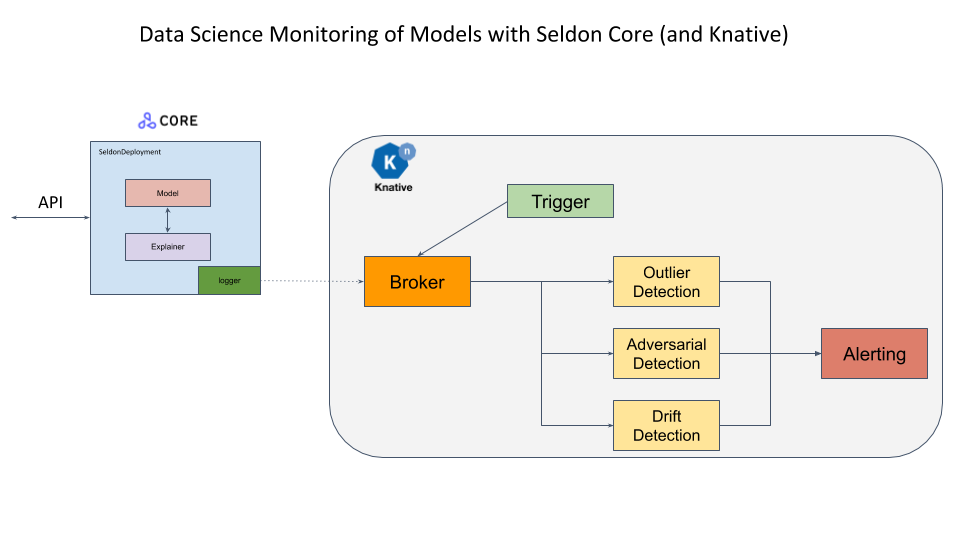
検知器を配備する
このサンプルのオープンソース配備プラットフォーム Seldon Core と (サーバレス・コンポーネントがイベントストリームに接続されることを可能にする) イベント・ベースのプロジェクト Knative を使用します。Seldon Core payload logger はモデルリクエストを含むイベントを Knative に送ります、これはこれらを外れ値、ドリフトや敵対的検知モジュールのようなサーバレス・コンポーネントに委託することができます。更に例えばアラート or ストレージ・モジュールに前方に送るためにこれらのコンポーネントにより生成されたイベントを供給するためにイベント・コンポーネントが追加できます。これらは非同期に発生します。
既に Seldon Core をインストールして DigitalOcean 上クラスタを構成しました。スクラッチから総てをセットアップする構成ステップは このサンプル・ノートブック で詳述されています。
最初に Istio Ingress Gatewaw の IP アドレスを取得します。これは Istio が LoadBalancer とともにインストールされていることを仮定しています。
CLUSTER_IPS=!(kubectl -n istio-system get service istio-ingressgateway -o jsonpath='{.status.loadBalancer.ingress[0].ip}')
CLUSTER_IP=CLUSTER_IPS[0]
print(CLUSTER_IP)
188.166.139.197
SERVICE_HOSTNAMES=!(kubectl get ksvc vae-outlier -o jsonpath='{.status.url}' | cut -d "/" -f 3)
SERVICE_HOSTNAME_VAEOD=SERVICE_HOSTNAMES[0]
print(SERVICE_HOSTNAME_VAEOD)
vae-outlier.default.example.com
配備されたモデルの予測のために幾つかのユティリティ関数を定義します。
import json
import requests
from typing import Union

classes = ('plane', 'car', 'bird', 'cat', 'deer',
           'dog', 'frog', 'horse', 'ship', 'truck')

def predict(x: np.ndarray) -> Union[str, list]:
    """ Model prediction. """
    formData = {
    'instances': x.tolist()
    }
    headers = {}
    res = requests.post(
        'http://'+CLUSTER_IP+'/seldon/default/tfserving-cifar10/v1/models/resnet32/:predict',
        json=formData,
        headers=headers
    )
    if res.status_code == 200:
        return classes[np.array(res.json()["predictions"])[0].argmax()]
    else:
        print("Failed with ",res.status_code)
        return []


def outlier(x: np.ndarray) -> Union[dict, list]:
    """ Outlier prediction. """
    formData = {
    'instances': x.tolist()
    }
    headers = {
        "Alibi-Detect-Return-Feature-Score": "true",
        "Alibi-Detect-Return-Instance-Score": "true"
    }
    headers["Host"] = SERVICE_HOSTNAME_VAEOD
    res = requests.post('http://'+CLUSTER_IP+'/', json=formData, headers=headers)
    if res.status_code == 200:
        od = res.json()
        od["data"]["feature_score"] = np.array(od["data"]["feature_score"])
        od["data"]["instance_score"] = np.array(od["data"]["instance_score"])
        return od
    else:
        print("Failed with ",res.status_code)
        return []


def show(x: np.ndarray) -> None:
    plt.imshow(x.reshape(32, 32, 3))
    plt.axis('off')
    plt.show()
元のインスタンス上で予測を行ないましょう :
show(x)
predict(x)

'ship'
外れ値検知器の出力のためにメッセージ dumper を確認しましょう :
res=!kubectl logs $(kubectl get pod -l serving.knative.dev/configuration=message-dumper -o jsonpath='{.items[0].metadata.name}') user-container
data = []
for i in range(0,len(res)):
    if res[i] == 'Data,':
        data.append(res[i+1])
j = json.loads(json.loads(data[0]))
print("Outlier?",labels[j["data"]["is_outlier"]==[1]])
Outlier? No!
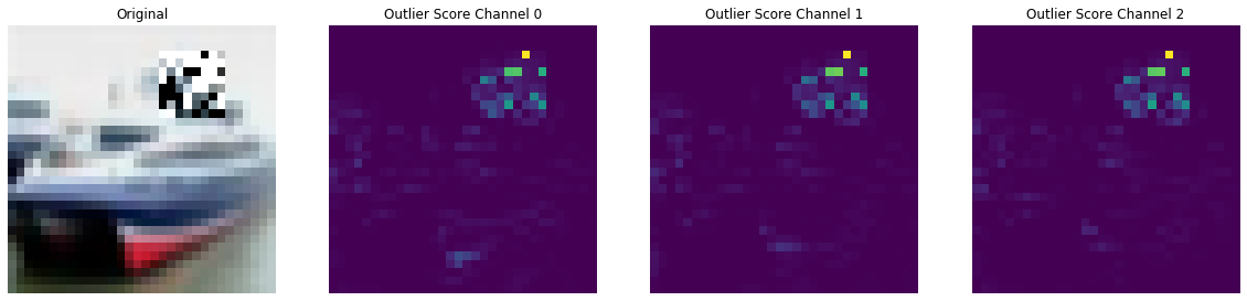
そして摂動されたインスタンスで予測を行ないます :
show(x_mask)
predict(x_mask)

'ship'
予測は依然として正しいですが、インスタンスは明らかに外れ値です :
res=!kubectl logs $(kubectl get pod -l serving.knative.dev/configuration=message-dumper -o jsonpath='{.items[0].metadata.name}') user-container
data= []
for i in range(0,len(res)):
    if res[i] == 'Data,':
        data.append(res[i+1])
j = json.loads(json.loads(data[1]))
print("Outlier?",labels[j["data"]["is_outlier"]==[1]])
Outlier? Yes!
preds = outlier(x_mask)
plot_feature_outlier_image(preds, x_mask, X_recon=None)
2. 予測確率のマッチングによる敵対的検知
メソッド
敵対的検知器は Adversarial Detection and Correction by Matching Prediction Distributions に基づいています。通常、オートエンコーダは平均二乗再構築誤差のような $x$ と $x’$ の間の類似性を捕捉するのに適する損失関数を用いて、入力インスタンス $x$ を出来る限り正確に再構築するような変換 $T$ を見つけるために訓練されます。敵対的オートエンコーダ (AE) 検知器の新奇性は、オートエンコーダネットワークを訓練するために、モデルの出力空間の距離尺度に基づいた分類モデル依存な損失関数の使用に依存していることです。分類モデル $M$ が与えられたとき、オートエンコーダの重みは $x$ と $x’$ のモデル予測間の KL-ダイバージェンス を最小化するように最適化されます。再構築損失項 $x’$ の存在がない場合には、$x$ と $x’$ の近接性を気に掛けることなく、単純に予測確率 $M(x’)$ と $M(x)$ が一致することを確かなものにしようとします。その結果、$x’$ はモデル $M$ に関する異なる決定境界 shape によって $x$ とは異なる入力特徴空間の異なる領域に存在することが可能になります。$x$ 周りで効果的な注意深く作成された敵対的摂動は特徴空間の $x’$ の新しい位置には転送されませんので、従って攻撃は無力化されます。オートエンコーダの訓練は教師なしです、何故ならばモデル予測確率と通常の訓練インスタンスへのアクセスだけを必要とするからです。基礎となる敵対的攻撃についての知識を必要としません、そして分類器の重みは訓練の間凍結されます。
検知器は以下のように利用できます :
- 敵対的スコア $S$ が計算されます。$S$ は $x$ と $x’$ のモデル予測間の K-L ダイバージェンスに等しいです。
- $S$ が (明示的に定義されたか訓練データから推論された) 閾値を越える場合、インスタンスは敵対的とフラグ立てされます。
- 敵対的インスタンスについては、モデル $M$ は予測を行なうために再構築されたインスタンス $x’$ を使用します。敵対的スコアが閾値の下であれば、モデルは元のインスタンス $x$ 上で予測を行ないます。
この手順は下の図で図示されます :
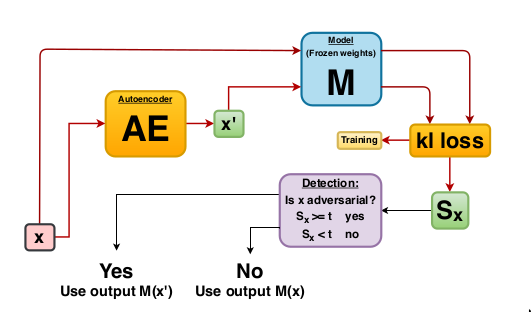
この方法は非常に柔軟で、モデル性能にネガティブな影響を与える一般的なデータ破損と摂動を検出するためにも使用できます。
# more imports
from sklearn.metrics import roc_curve, auc
from alibi_detect.ad import AdversarialAE
from alibi_detect.datasets import fetch_attack
from alibi_detect.utils.fetching import fetch_tf_model
from alibi_detect.utils.prediction import predict_batch
ユティリティ関数
# instance scaling and plotting utility functions
def scale_by_instance(X: np.ndarray) -> np.ndarray:
    mean_ = X.mean(axis=(1, 2, 3)).reshape(-1, 1, 1, 1)
    std_ = X.std(axis=(1, 2, 3)).reshape(-1, 1, 1, 1)
    return (X - mean_) / std_, mean_, std_


def accuracy(y_true: np.ndarray, y_pred: np.ndarray) -> float:
    return (y_true == y_pred).astype(int).sum() / y_true.shape[0]


def plot_adversarial(idx: list,
                     X: np.ndarray,
                     y: np.ndarray,
                     X_adv: np.ndarray,
                     y_adv: np.ndarray,
                     mean: np.ndarray,
                     std: np.ndarray,
                     score_x: np.ndarray = None,
                     score_x_adv: np.ndarray = None,
                     X_recon: np.ndarray = None,
                     y_recon: np.ndarray = None,
                     figsize: tuple = (10, 5)) -> None:

    # category map from class numbers to names
    cifar10_map = {0: 'airplane', 1: 'automobile', 2: 'bird', 3: 'cat', 4: 'deer', 5: 'dog',
                   6: 'frog', 7: 'horse', 8: 'ship', 9: 'truck'}

    nrows = len(idx)
    ncols = 3 if isinstance(X_recon, np.ndarray) else 2
    fig, ax = plt.subplots(nrows=nrows, ncols=ncols, figsize=figsize)

    n_subplot = 1
    for i in idx:

        # rescale images in [0, 1]
        X_adj = (X[i] * std[i] + mean[i]) / 255
        X_adv_adj = (X_adv[i] * std[i] + mean[i]) / 255
        if isinstance(X_recon, np.ndarray):
            X_recon_adj = (X_recon[i] * std[i] + mean[i]) / 255

        # original image
        plt.subplot(nrows, ncols, n_subplot)
        plt.axis('off')
        if i == idx[0]:
            if isinstance(score_x, np.ndarray):
                plt.title('CIFAR-10 Image \n{}: {:.3f}'.format(cifar10_map[y[i]], score_x[i]))
            else:
                plt.title('CIFAR-10 Image \n{}'.format(cifar10_map[y[i]]))
        else:
            if isinstance(score_x, np.ndarray):
                plt.title('{}: {:.3f}'.format(cifar10_map[y[i]], score_x[i]))
            else:
                plt.title('{}'.format(cifar10_map[y[i]]))
        plt.imshow(X_adj)
        n_subplot += 1

        # adversarial image
        plt.subplot(nrows, ncols, n_subplot)
        plt.axis('off')
        if i == idx[0]:
            if isinstance(score_x_adv, np.ndarray):
                plt.title('Adversarial \n{}: {:.3f}'.format(cifar10_map[y_adv[i]], score_x_adv[i]))
            else:
                plt.title('Adversarial \n{}'.format(cifar10_map[y_adv[i]]))
        else:
            if isinstance(score_x_adv, np.ndarray):
                plt.title('{}: {:.3f}'.format(cifar10_map[y_adv[i]], score_x_adv[i]))
            else:
                plt.title('{}'.format(cifar10_map[y_adv[i]]))
        plt.imshow(X_adv_adj)
        n_subplot += 1

        # reconstructed image
        if isinstance(X_recon, np.ndarray):
            plt.subplot(nrows, ncols, n_subplot)
            plt.axis('off')
            if i == idx[0]:
                plt.title('AE Reconstruction \n{}'.format(cifar10_map[y_recon[i]]))
            else:
                plt.title('{}'.format(cifar10_map[y_recon[i]]))
            plt.imshow(X_recon_adj)
            n_subplot += 1

    plt.show()


def plot_roc(roc_data: dict, figsize: tuple = (10,5)):
    plot_labels = []
    scores_attacks = []
    labels_attacks = []
    for k, v in roc_data.items():
        if 'original' in k:
            continue
        score_x = roc_data[v['normal']]['scores']
        y_pred = roc_data[v['normal']]['predictions']
        score_v = v['scores']
        y_pred_v = v['predictions']
        labels_v = np.ones(score_x.shape[0])
        idx_remove = np.where(y_pred == y_pred_v)[0]
        labels_v = np.delete(labels_v, idx_remove)
        score_v = np.delete(score_v, idx_remove)
        scores = np.concatenate([score_x, score_v])
        labels = np.concatenate([np.zeros(y_pred.shape[0]), labels_v]).astype(int)
        scores_attacks.append(scores)
        labels_attacks.append(labels)
        plot_labels.append(k)

    for sc_att, la_att, plt_la in zip(scores_attacks, labels_attacks, plot_labels):
        fpr, tpr, thresholds = roc_curve(la_att, sc_att)
        roc_auc = auc(fpr, tpr)
        label = str('{}: AUC = {:.2f}'.format(plt_la, roc_auc))
        plt.plot(fpr, tpr, lw=1, label='{}: AUC={:.4f}'.format(plt_la, roc_auc))

    plt.plot([0, 1], [0, 1], color='black', lw=1, linestyle='--')
    plt.xlim([0.0, 1.0])
    plt.ylim([0.0, 1.05])
    plt.xlabel('False Positive Rate')
    plt.ylabel('True Positive Rate')
    plt.title('{}'.format('ROC curve'))
    plt.legend(loc="lower right", ncol=1)
    plt.grid()
    plt.show()
データをリスケールする
ResNet 分類モデルはインスタンスにより標準化されたデータ上で訓練されます :
# rescale data
X_train, mean_train, std_train = scale_by_instance(X_train * 255.)
X_test, mean_test, std_test = scale_by_instance(X_test * 255.)
scale = (mean_train, std_train), (mean_test, std_test)
事前訓練済みの分類器をロードする
dataset = 'cifar10'
model = 'resnet56'
clf = fetch_tf_model(dataset, model)
テスト上の予測を確認します :
y_pred = predict_batch(clf, X_test, batch_size=32, return_class=True)
acc_y_pred = accuracy(y_test, y_pred)
print('Accuracy: {:.4f}'.format(acc_y_pred))
Accuracy: 0.9315
敵対的攻撃
Carlini-Wagner (C&W) と SLIDE 攻撃の両者を調査します。以前に見つかった敵対的なインスタンスを事前訓練済みの ResNet-56 モデル上に単純にロードできます。攻撃は Foolbox を使用して生成されます :
# C&W attack
data_cw = fetch_attack(dataset, model, 'cw')
X_train_cw, X_test_cw = data_cw['data_train'], data_cw['data_test']
meta_cw = data_cw['meta'] # metadata with hyperparameters of the attack
# SLIDE attack
data_slide = fetch_attack(dataset, model, 'slide')
X_train_slide, X_test_slide = data_slide['data_train'], data_slide['data_test']
meta_slide = data_slide['meta']
分類器の精度が殆ど 0% に低下することを検証できます :
y_pred_cw = predict_batch(clf, X_test_cw, batch_size=32, return_class=True)
y_pred_slide = predict_batch(clf, X_test_slide, batch_size=32, return_class=True)
acc_y_pred_cw = accuracy(y_test, y_pred_cw)
acc_y_pred_slide = accuracy(y_test, y_pred_slide)
print('Accuracy: cw {:.4f} -- SLIDE {:.4f}'.format(acc_y_pred_cw, acc_y_pred_slide))
Accuracy: cw 0.0000 -- SLIDE 0.0001
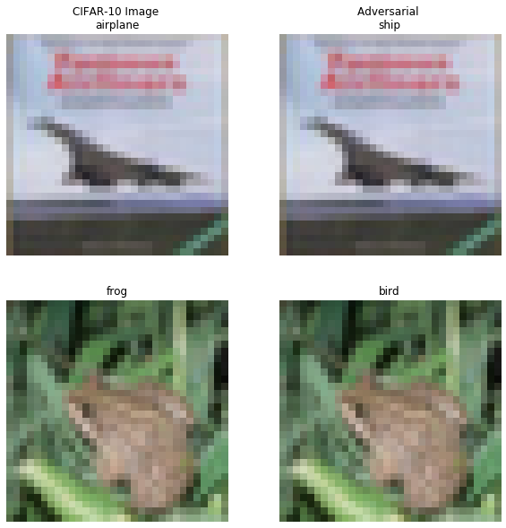
幾つかの敵対的インスタンスを可視化しましょう :
# plot attacked instances
idx = [3, 4]
print('C&W attack...')
plot_adversarial(idx, X_test, y_pred, X_test_cw, y_pred_cw,
                 mean_test, std_test, figsize=(10, 10))
print('SLIDE attack...')
plot_adversarial(idx, X_test, y_pred, X_test_slide, y_pred_slide,
                 mean_test, std_test, figsize=(10, 10))
C&W 攻撃 …

SLIDE 攻撃 …
敵対的検知器をロードまたは訓練して評価する
Google Cloud Bucket から事前訓練済みの検知器を再度取得するかスクラッチから訓練できます :
load_pretrained = False
filepath = os.path.join(os.getcwd(), 'adversarial')

if load_pretrained:
    detector_type = 'adversarial'
    detector_name = 'base'
    ad = fetch_detector(filepath, detector_type, dataset, detector_name, model=model)
    filepath = os.path.join(filepath, detector_name)
else:  # train detector from scratch

    # define encoder and decoder networks
    encoder_net = tf.keras.Sequential(
            [
                InputLayer(input_shape=(32, 32, 3)),
                Conv2D(32, 4, strides=2, padding='same',
                       activation=tf.nn.relu, kernel_regularizer=l1(1e-5)),
                Conv2D(64, 4, strides=2, padding='same',
                       activation=tf.nn.relu, kernel_regularizer=l1(1e-5)),
                Conv2D(256, 4, strides=2, padding='same',
                       activation=tf.nn.relu, kernel_regularizer=l1(1e-5)),
                Flatten(),
                Dense(40)
            ]
        )

    decoder_net = tf.keras.Sequential(
        [
                InputLayer(input_shape=(40,)),
                Dense(4 * 4 * 128, activation=tf.nn.relu),
                Reshape(target_shape=(4, 4, 128)),
                Conv2DTranspose(256, 4, strides=2, padding='same',
                                activation=tf.nn.relu, kernel_regularizer=l1(1e-5)),
                Conv2DTranspose(64, 4, strides=2, padding='same',
                                activation=tf.nn.relu, kernel_regularizer=l1(1e-5)),
                Conv2DTranspose(3, 4, strides=2, padding='same',
                                activation=None, kernel_regularizer=l1(1e-5))
            ]
        )

    # initialise and train detector
    ad = AdversarialAE(
        encoder_net=encoder_net,
        decoder_net=decoder_net,
        model=clf
    )
    ad.fit(X_train, epochs=40, batch_size=64, verbose=True)

    # save the trained adversarial detector
    save_detector(ad, filepath)
検知器は最初に敵対的であり得る入力インスタンスを再構築します。そして再構築された入力は敵対的スコアを計算するために分類器に供給されます。スコアが閾値より上の場合、インスタンスは敵対的と分類されて検知器は攻撃を正そうとします。攻撃されたインスタンスを再構築してその上で予測を行なうとき何が起きるかを調べましょう :
X_recon_cw = predict_batch(ad.ae, X_test_cw, batch_size=32)
X_recon_slide = predict_batch(ad.ae, X_test_slide, batch_size=32)
y_recon_cw = predict_batch(clf, X_recon_cw, batch_size=32, return_class=True)
y_recon_slide = predict_batch(clf, X_recon_slide, batch_size=32, return_class=True)
攻撃された (インスタンス) vs. 再構築されたインスタンスの精度 :
acc_y_recon_cw = accuracy(y_test, y_recon_cw)
acc_y_recon_slide = accuracy(y_test, y_recon_slide)
print('Accuracy after C&W attack {:.4f} -- reconstruction {:.4f}'.format(acc_y_pred_cw, acc_y_recon_cw))
print('Accuracy after SLIDE attack {:.4f} -- reconstruction {:.4f}'.format(acc_y_pred_slide, acc_y_recon_slide))
Accuracy after C&W attack 0.0000 -- reconstruction 0.8048
Accuracy after SLIDE attack 0.0001 -- reconstruction 0.8159
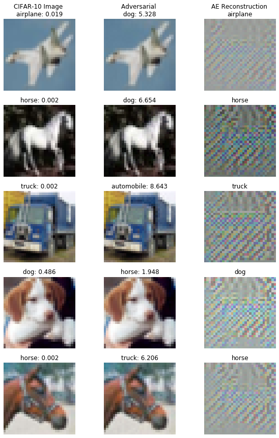
検知器は攻撃後の精度を殆ど 0 % から 80% を上手く越えるまでに復旧します!攻撃的スコアを計算して再構築されたインスタンスの幾つかを調査できます :
score_x = ad.score(X_test, batch_size=32)
score_cw = ad.score(X_test_cw, batch_size=32)
score_slide = ad.score(X_test_slide, batch_size=32)
# visualize original, attacked and reconstructed instances with adversarial scores
print('C&W attack...')
idx = [10, 13, 14, 16, 17]
plot_adversarial(idx, X_test, y_pred, X_test_cw, y_pred_cw, mean_test, std_test,
score_x=score_x, score_x_adv=score_cw, X_recon=X_recon_cw,
y_recon=y_recon_cw, figsize=(10, 15))
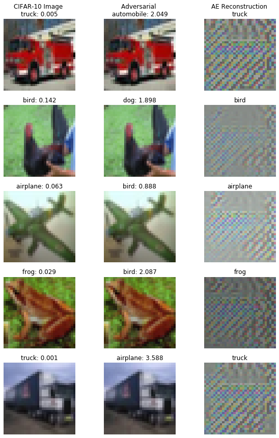
print('SLIDE attack...')
idx = [23, 25, 27, 29, 34]
plot_adversarial(idx, X_test, y_pred, X_test_slide, y_pred_slide, mean_test, std_test,
score_x=score_x, score_x_adv=score_slide, X_recon=X_recon_slide,
y_recon=y_recon_slide, figsize=(10, 15))
C&W 攻撃 …
SLIDE 攻撃 …
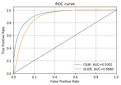
ROC カーブと AUC 値は敵対的インスタンスを検知するための敵対的スコアの有効性を示します :
# plot roc curve
roc_data = {
    'original': {'scores': score_x, 'predictions': y_pred},
    'C&W': {'scores': score_cw, 'predictions': y_pred_cw, 'normal': 'original'},
    'SLIDE': {'scores': score_slide, 'predictions': y_pred_slide, 'normal': 'original'}
}

plot_roc(roc_data)
敵対的スコアのための閾値は infer_threshold を通して設定できます。インスタンスのバッチ X を渡してそれらの何パーセントを正常であると考えるかを threshold_perc を通して指定する必要があります。Assume we have only normal instances some of which the model has misclassified leading to a higher score if the reconstruction picked up features from the correct class or some might look adversarial in the first place. その結果、閾値を 95% に設定します :
ad.infer_threshold(X_test, threshold_perc=95, margin=0., batch_size=32)
print('Adversarial threshold: {:.4f}'.format(ad.threshold))
Adversarial threshold: 2.6722
検知器の正しい方法は Figure 1 の図を実行します。最初に敵対的スコアが計算されます。スコアが閾値を越えるインスタンスについては、再構築されたインスタンスの分類器予測が返されます。そうでなければ元の予測が保持されます。このメソッドは検知器のメタデータ、(バッチのインスタンスが敵対的であろうとなかろうと、) 訂正メカニズムを使用した分類器予測、そして元の予測と再構築された予測の両者を含む辞書を返します。幾つかの敵対的 (インスタンス) そして元のテストセットのインスタンスを含むバッチでこれを示しましょう :
n_test = X_test.shape[0]
np.random.seed(0)
idx_normal = np.random.choice(n_test, size=1600, replace=False)
idx_cw = np.random.choice(n_test, size=400, replace=False)

X_mix = np.concatenate([X_test[idx_normal], X_test_cw[idx_cw]])
y_mix = np.concatenate([y_test[idx_normal], y_test[idx_cw]])
print(X_mix.shape, y_mix.shape)
(2000, 32, 32, 3) (2000,)
モデル性能を確認しましょう :
y_pred_mix = predict_batch(clf, X_mix, batch_size=32, return_class=True)
acc_y_pred_mix = accuracy(y_mix, y_pred_mix)
print('Accuracy {:.4f}'.format(acc_y_pred_mix))
Accuracy 0.7380
これは訂正メカニズムで改良できます :
preds = ad.correct(X_mix, batch_size=32)
acc_y_corr_mix = accuracy(y_mix, preds['data']['corrected'])
print('Accuracy {:.4f}'.format(acc_y_corr_mix))
Accuracy 0.8205
論文 でハイライトされていて (temperature スケーリング と 隠れ層 K-L ダイバージェンス) Alibi Detect で実装されている幾つかの他のトリックがあります、これは敵対的検知器の性能を更にブーストできます。より詳細については この example ノートブック を確認してください。
以上
Alibi Detect 0.7 : Examples : AE 外れ値検知 on CIFAR10
Alibi Detect 0.7 : Examples : AE 外れ値検知 on CIFAR10 (翻訳/解説)
翻訳 : (株)クラスキャット セールスインフォメーション
作成日時 : 07/04/2021 (0.7.0)
* 本ページは、Alibi Detect の以下のドキュメントを翻訳した上で適宜、補足説明したものです:
* サンプルコードの動作確認はしておりますが、必要な場合には適宜、追加改変しています。
* ご自由にリンクを張って頂いてかまいませんが、sales-info@classcat.com までご一報いただけると嬉しいです。
スケジュールは弊社 公式 Web サイト でご確認頂けます。
- お住まいの地域に関係なく Web ブラウザからご参加頂けます。事前登録 が必要ですのでご注意ください。
- ウェビナー運用には弊社製品「ClassCat® Webinar」を利用しています。
| 人工知能研究開発支援 | 人工知能研修サービス | テレワーク & オンライン授業を支援 |
| PoC(概念実証)を失敗させないための支援 (本支援はセミナーに参加しアンケートに回答した方を対象としています。) | ||
◆ お問合せ : 本件に関するお問い合わせ先は下記までお願いいたします。
| 株式会社クラスキャット セールス・マーケティング本部 セールス・インフォメーション |
| E-Mail:sales-info@classcat.com ; WebSite: https://www.classcat.com/ ; Facebook |
Alibi Detect 0.7 : Examples : AE 外れ値検知 on CIFAR10
オートエンコーダ – 概要
オートエンコーダ (AE, Auto-Encoder) 外れ値検知器はラベル付けされていない、しかし通常 (inlier) データのバッチで最初に訓練されます。教師なし訓練が望ましいです、何故ならばラベル付けされたデータはしばしば十分でないからです。AE 検知器はそれが受け取る入力を再構築しようとします。入力データが上手く再構築されない場合、再構築エラーは高くそしてデータは外れ値としてフラグ立てできます。再構築エラーは入力と再構築されたインスタンスの間の平均二乗誤差 (MSE, mean squared error) として測定されます。
データセット
CIFAR10 は 10 クラスに渡り均等に分配された 60,000 の 32 x 32 RGB 画像から成ります。
import logging
import matplotlib.pyplot as plt
import numpy as np
import os
import tensorflow as tf
tf.keras.backend.clear_session()
from tensorflow.keras.layers import Conv2D, Conv2DTranspose, \
    Dense, Layer, Reshape, InputLayer, Flatten
from tqdm import tqdm

from alibi_detect.od import OutlierAE
from alibi_detect.utils.fetching import fetch_detector
from alibi_detect.utils.perturbation import apply_mask
from alibi_detect.utils.saving import save_detector, load_detector
from alibi_detect.utils.visualize import plot_instance_score, plot_feature_outlier_image

logger = tf.get_logger()
logger.setLevel(logging.ERROR)
CIFAR10 データをロードする
train, test = tf.keras.datasets.cifar10.load_data()
X_train, y_train = train
X_test, y_test = test

X_train = X_train.astype('float32') / 255
X_test = X_test.astype('float32') / 255
print(X_train.shape, y_train.shape, X_test.shape, y_test.shape)
(50000, 32, 32, 3) (50000, 1) (10000, 32, 32, 3) (10000, 1)
外れ値検知器をロードまたは定義する
examples ノートブックで使用される事前訓練済みの外れ値と敵対的検知器は ここ で見つかります。組込みの fetch_detector 関数を利用できます、これは事前訓練モデルをローカルディレクトリ filepath にセーブして検知器をロードします。代わりに、スクラッチから検知器を訓練することができます :
load_outlier_detector = False
filepath = 'model_ae_cifar10'  # change to (absolute) directory where model is downloaded
if load_outlier_detector:  # load pretrained outlier detector
    detector_type = 'outlier'
    dataset = 'cifar10'
    detector_name = 'OutlierAE'
    od = fetch_detector(filepath, detector_type, dataset, detector_name)
    filepath = os.path.join(filepath, detector_name)
else:  # define model, initialize, train and save outlier detector
    encoding_dim = 1024

    encoder_net = tf.keras.Sequential(
      [
          InputLayer(input_shape=(32, 32, 3)),
          Conv2D(64, 4, strides=2, padding='same', activation=tf.nn.relu),
          Conv2D(128, 4, strides=2, padding='same', activation=tf.nn.relu),
          Conv2D(512, 4, strides=2, padding='same', activation=tf.nn.relu),
          Flatten(),
          Dense(encoding_dim,)
      ])

    decoder_net = tf.keras.Sequential(
      [
          InputLayer(input_shape=(encoding_dim,)),
          Dense(4*4*128),
          Reshape(target_shape=(4, 4, 128)),
          Conv2DTranspose(256, 4, strides=2, padding='same', activation=tf.nn.relu),
          Conv2DTranspose(64, 4, strides=2, padding='same', activation=tf.nn.relu),
          Conv2DTranspose(3, 4, strides=2, padding='same', activation='sigmoid')
      ])

    # initialize outlier detector
    od = OutlierAE(threshold=.015,  # threshold for outlier score
                    encoder_net=encoder_net,  # can also pass AE model instead
                    decoder_net=decoder_net,  # of separate encoder and decoder
                    )
    # train
    od.fit(X_train,
           epochs=50,
           verbose=True)

    # save the trained outlier detector
    save_detector(od, filepath)
AE モデルの品質を確認する
idx = 8
X = X_train[idx].reshape(1, 32, 32, 3)
X_recon = od.ae(X)
plt.imshow(X.reshape(32, 32, 3))
plt.axis('off')
plt.show()

plt.imshow(X_recon.numpy().reshape(32, 32, 3))
plt.axis('off')
plt.show()

元の CIFAR10 画像の外れ値を確認する
X = X_train[:500]
print(X.shape)
(500, 32, 32, 3)
od_preds = od.predict(X,
                      outlier_type='instance',    # use 'feature' or 'instance' level
                      return_feature_score=True,  # scores used to determine outliers
                      return_instance_score=True)
print(list(od_preds['data'].keys()))
['instance_score', 'feature_score', 'is_outlier']
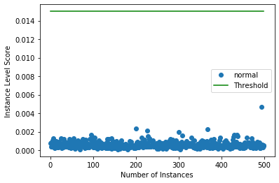
インスタンスレベルの外れ値スコアをプロットする
target = np.zeros(X.shape[0],).astype(int)  # all normal CIFAR10 training instances
labels = ['normal', 'outlier']
plot_instance_score(od_preds, target, labels, od.threshold)
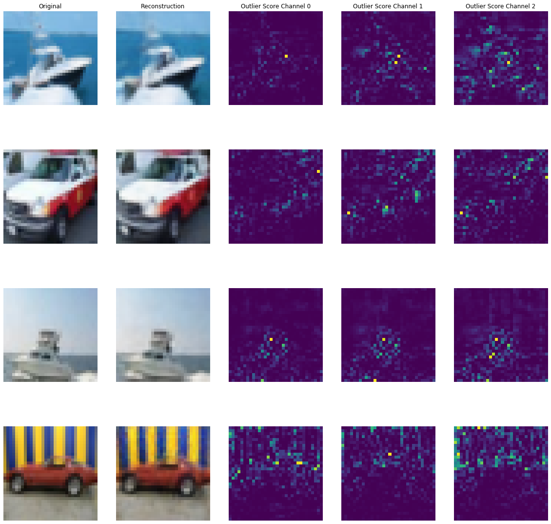
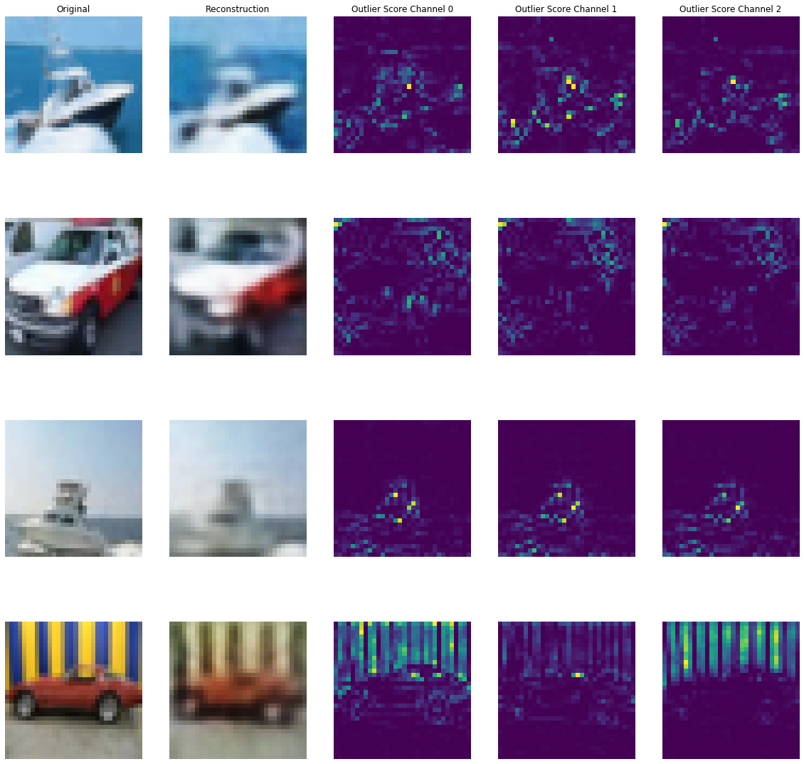
予測を可視化する
X_recon = od.ae(X).numpy()
plot_feature_outlier_image(od_preds,
                           X,
                           X_recon=X_recon,
                           instance_ids=[8, 60, 100, 330],  # pass a list with indices of instances to display
                           max_instances=5,  # max nb of instances to display
                           outliers_only=False)  # only show outlier predictions
摂動された CIFAR 画像で外れ値を予測する
CIFAR 画像を画像のパッチ (マスク) にランダムノイズを追加することにより摂動させます。n_mask_sizes の各マスクサイズについて、n_masks をサンプリングしてそれらを n_imgs 画像の各々に適用します。そしてマスクされたインスタンスで外れ値を予測します :
# nb of predictions per image: n_masks * n_mask_sizes
n_mask_sizes = 10
n_masks = 20
n_imgs = 50
マスクを定義して画像を取得します :
mask_sizes = [(2*n,2*n) for n in range(1,n_mask_sizes+1)]
print(mask_sizes)
img_ids = np.arange(n_imgs)
X_orig = X[img_ids].reshape(img_ids.shape[0], 32, 32, 3)
print(X_orig.shape)
[(2, 2), (4, 4), (6, 6), (8, 8), (10, 10), (12, 12), (14, 14), (16, 16), (18, 18), (20, 20)]
(50, 32, 32, 3)
インスタンスレベルの外れ値スコアを計算します :
all_img_scores = []
for i in tqdm(range(X_orig.shape[0])):
    img_scores = np.zeros((len(mask_sizes),))
    for j, mask_size in enumerate(mask_sizes):
        # create masked instances
        X_mask, mask = apply_mask(X_orig[i].reshape(1, 32, 32, 3),
                                  mask_size=mask_size,
                                  n_masks=n_masks,
                                  channels=[0,1,2],
                                  mask_type='normal',
                                  noise_distr=(0,1),
                                  clip_rng=(0,1))
        # predict outliers
        od_preds_mask = od.predict(X_mask)
        score = od_preds_mask['data']['instance_score']
        # store average score over `n_masks` for a given mask size
        img_scores[j] = np.mean(score)
    all_img_scores.append(img_scores)
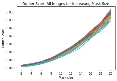
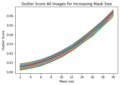
外れ値スコア vs. マスクサイズを可視化する
x_plt = [mask[0] for mask in mask_sizes]
for ais in all_img_scores:
    plt.plot(x_plt, ais)
    plt.xticks(x_plt)
plt.title('Outlier Score All Images for Increasing Mask Size')
plt.xlabel('Mask size')
plt.ylabel('Outlier Score')
plt.show()
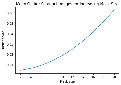
ais_np = np.zeros((len(all_img_scores), all_img_scores[0].shape[0]))
for i, ais in enumerate(all_img_scores):
ais_np[i, :] = ais
ais_mean = np.mean(ais_np, axis=0)
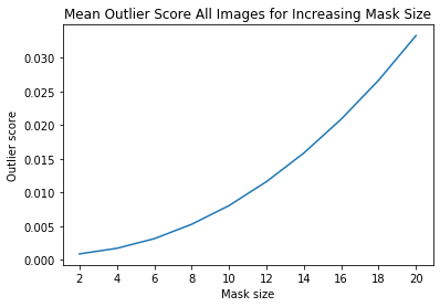
plt.title('Mean Outlier Score All Images for Increasing Mask Size')
plt.xlabel('Mask size')
plt.ylabel('Outlier score')
plt.plot(x_plt, ais_mean)
plt.xticks(x_plt)
plt.show()
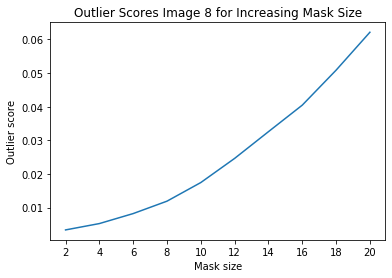
インスタンスレベルの外れ値を調査する
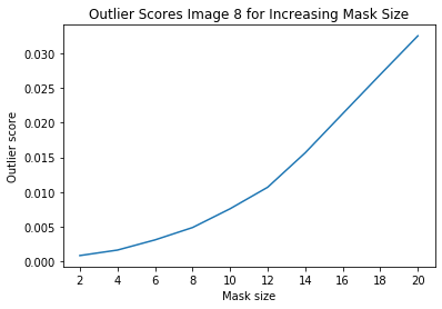
i = 8 # index of instance to look at
plt.plot(x_plt, all_img_scores[i])
plt.xticks(x_plt)
plt.title('Outlier Scores Image {} for Increasing Mask Size'.format(i))
plt.xlabel('Mask size')
plt.ylabel('Outlier score')
plt.show()
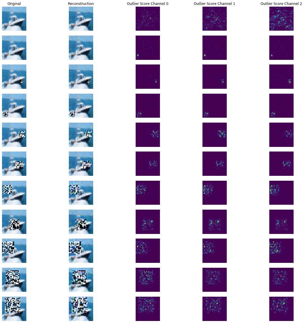
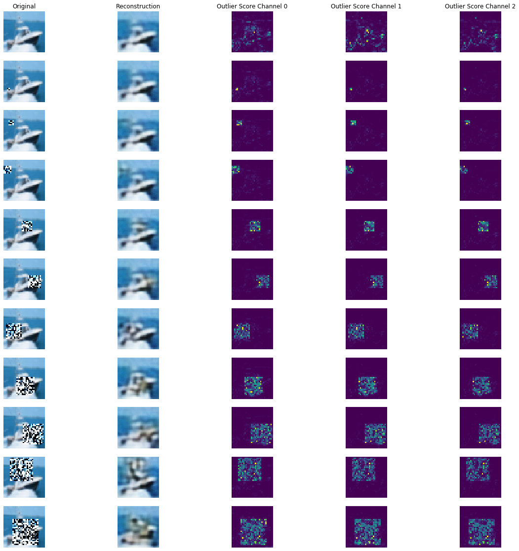
マスクされた画像の再構築とチャネル毎の外れ値スコア :
all_X_mask = []
X_i = X_orig[i].reshape(1, 32, 32, 3)
all_X_mask.append(X_i)
# apply masks
for j, mask_size in enumerate(mask_sizes):
    # create masked instances
    X_mask, mask = apply_mask(X_i,
                              mask_size=mask_size,
                              n_masks=1,  # just 1 for visualization purposes
                              channels=[0,1,2],
                              mask_type='normal',
                              noise_distr=(0,1),
                              clip_rng=(0,1))
    all_X_mask.append(X_mask)
all_X_mask = np.concatenate(all_X_mask, axis=0)
all_X_recon = od.ae(all_X_mask).numpy()
od_preds = od.predict(all_X_mask)
可視化します :
plot_feature_outlier_image(od_preds,
                           all_X_mask,
                           X_recon=all_X_recon,
                           max_instances=all_X_mask.shape[0],
                           n_channels=3)
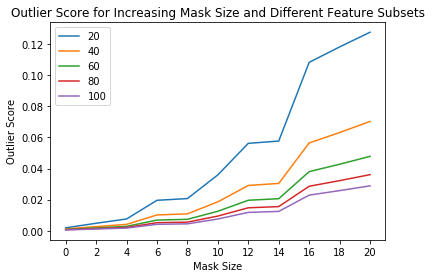
特徴のサブセットで外れ値を予測する
外れ値検知器の sensitivity (感度) は閾値を通してだけでなくインスタンスレベルの外れ値スコア計算のために使用される特徴のパーセンテージを選択することによっても制御できます。例えば、特徴の 40% が閾値を越える平均外れ値スコアを持つ場合外れ値であるとフラグ立てすることを望むかもしれません。これは predict 関数の outlier_perc 引数を通して可能です。それは降順の外れ値スコア順序でソートされた、外れ値検知のために使用される特徴のパーセンテージを指定します。
perc_list = [20, 40, 60, 80, 100]

all_perc_scores = []
for perc in perc_list:
    od_preds_perc = od.predict(all_X_mask, outlier_perc=perc)
    iscore = od_preds_perc['data']['instance_score']
    all_perc_scores.append(iscore)
外れ値スコア vs. マスクサイズと使用された特徴サイズのパーセンテージを可視化します :
x_plt = [0] + x_plt
for aps in all_perc_scores:
    plt.plot(x_plt, aps)
    plt.xticks(x_plt)
plt.legend(perc_list)
plt.title('Outlier Score for Increasing Mask Size and Different Feature Subsets')
plt.xlabel('Mask Size')
plt.ylabel('Outlier Score')
plt.show()
外れ値の閾値を推論する
良い閾値を見つけることは技巧的であり得ます、何故ならばそれらは典型的には解釈することが容易でないからです。infer_threshold メソッドは sensible な値を見つけるのに役立ちます。インスタンスのバッチ X を渡してそれらの何パーセントを正常であると考えるかを threshold_perc を通して指定する必要があります。
print('Current threshold: {}'.format(od.threshold))
od.infer_threshold(X, threshold_perc=99)  # assume 1% of the training data are outliers
print('New threshold: {}'.format(od.threshold))
Current threshold: 0.015
New threshold: 0.0017021061840932791
以上
Alibi Detect 0.7 : Examples : VAE 外れ値検知 on CIFAR10
Alibi Detect 0.7 : Examples : VAE 外れ値検知 on CIFAR10 (翻訳/解説)
翻訳 : (株)クラスキャット セールスインフォメーション
作成日時 : 07/04/2021 (0.7.0)
* 本ページは、Alibi Detect の以下のドキュメントを翻訳した上で適宜、補足説明したものです:
* サンプルコードの動作確認はしておりますが、必要な場合には適宜、追加改変しています。
* ご自由にリンクを張って頂いてかまいませんが、sales-info@classcat.com までご一報いただけると嬉しいです。
スケジュールは弊社 公式 Web サイト でご確認頂けます。
- お住まいの地域に関係なく Web ブラウザからご参加頂けます。事前登録 が必要ですのでご注意ください。
- ウェビナー運用には弊社製品「ClassCat® Webinar」を利用しています。
| 人工知能研究開発支援 | 人工知能研修サービス | テレワーク & オンライン授業を支援 |
| PoC(概念実証)を失敗させないための支援 (本支援はセミナーに参加しアンケートに回答した方を対象としています。) | ||
◆ お問合せ : 本件に関するお問い合わせ先は下記までお願いいたします。
| 株式会社クラスキャット セールス・マーケティング本部 セールス・インフォメーション |
| E-Mail:sales-info@classcat.com ; WebSite: https://www.classcat.com/ ; Facebook |

Alibi Detect 0.7 : Examples : VAE 外れ値検知 on CIFAR10
VAE – 概要
変分オートエンコーダ (VAE, Variational Auto-Encoder) 外れ値検知器は最初にラベル付けされていない、しかし通常 (inlier) データのバッチで訓練されます。教師なしか半教師あり訓練が望ましいです、何故ならばラベル付けされたデータはしばしば十分でないからです。VAE 検知器はそれが受け取る入力を再構築しようとします。入力データが上手く再構築されない場合、再構築エラーは高くそしてデータは外れ値としてフラグ立てできます。再構築エラーは、入力と再構築されたインスタンスの間の平均二乗誤差 (MSE, mean squared error) か、入力と再構築されたインスタンスの両者が同じプロセスで生成される確率として測定されます。アルゴリズムは表形式か画像データのために適合します。
データセット
CIFAR10 は 10 クラスに渡り均等に分配された 60,000 の 32 x 32 RGB 画像から成ります。
import logging
import matplotlib.pyplot as plt
import numpy as np
import tensorflow as tf
tf.keras.backend.clear_session()
from tensorflow.keras.layers import Conv2D, Conv2DTranspose, Dense, Layer, Reshape, InputLayer
from tqdm import tqdm

from alibi_detect.models.tensorflow.losses import elbo
from alibi_detect.od import OutlierVAE
from alibi_detect.utils.fetching import fetch_detector
from alibi_detect.utils.perturbation import apply_mask
from alibi_detect.utils.saving import save_detector, load_detector
from alibi_detect.utils.visualize import plot_instance_score, plot_feature_outlier_image

logger = tf.get_logger()
logger.setLevel(logging.ERROR)
CIFAR10 データをロードする
train, test = tf.keras.datasets.cifar10.load_data()
X_train, y_train = train
X_test, y_test = test

X_train = X_train.astype('float32') / 255
X_test = X_test.astype('float32') / 255
print(X_train.shape, y_train.shape, X_test.shape, y_test.shape)
(50000, 32, 32, 3) (50000, 1) (10000, 32, 32, 3) (10000, 1)
外れ値検知器をロードまたは定義する
examples ノートブックで使用される事前訓練済みの外れ値と敵対的検知器は ここ で見つかります。組込みの fetch_detector 関数を利用できます、これは事前訓練モデルをローカルディレクトリ filepath にセーブして検知器をロードします。代わりに、スクラッチから検知器を訓練することができます :
load_outlier_detector = False
filepath = 'model_vae_cifar10'  # change to directory where model is downloaded
if load_outlier_detector:  # load pretrained outlier detector
    detector_type = 'outlier'
    dataset = 'cifar10'
    detector_name = 'OutlierVAE'
    od = fetch_detector(filepath, detector_type, dataset, detector_name)
    filepath = os.path.join(filepath, detector_name)
else:  # define model, initialize, train and save outlier detector
    latent_dim = 1024

    encoder_net = tf.keras.Sequential(
      [
          InputLayer(input_shape=(32, 32, 3)),
          Conv2D(64, 4, strides=2, padding='same', activation=tf.nn.relu),
          Conv2D(128, 4, strides=2, padding='same', activation=tf.nn.relu),
          Conv2D(512, 4, strides=2, padding='same', activation=tf.nn.relu)
      ])

    decoder_net = tf.keras.Sequential(
      [
          InputLayer(input_shape=(latent_dim,)),
          Dense(4*4*128),
          Reshape(target_shape=(4, 4, 128)),
          Conv2DTranspose(256, 4, strides=2, padding='same', activation=tf.nn.relu),
          Conv2DTranspose(64, 4, strides=2, padding='same', activation=tf.nn.relu),
          Conv2DTranspose(3, 4, strides=2, padding='same', activation='sigmoid')
      ])

    # initialize outlier detector
    od = OutlierVAE(threshold=.015,  # threshold for outlier score
                    score_type='mse',  # use MSE of reconstruction error for outlier detection
                    encoder_net=encoder_net,  # can also pass VAE model instead
                    decoder_net=decoder_net,  # of separate encoder and decoder
                    latent_dim=latent_dim,
                    samples=2)
    # train
    od.fit(X_train,
           loss_fn=elbo,
           cov_elbo=dict(sim=.05),
           epochs=50,
           verbose=True)

    # save the trained outlier detector
    save_detector(od, filepath)
(訳注 : TF 2.5.0, 8 vCPUs)
782/782 [=] - 200s 254ms/step - loss: 3261.4951
782/782 [=] - 199s 254ms/step - loss: -2490.5888
782/782 [=] - 199s 254ms/step - loss: -3502.6840
782/782 [=] - 203s 259ms/step - loss: -3973.3844
782/782 [=] - 203s 259ms/step - loss: -4287.5373
782/782 [=] - 202s 258ms/step - loss: -4530.9941
782/782 [=] - 202s 257ms/step - loss: -4697.7253
782/782 [=] - 202s 257ms/step - loss: -4847.7671
782/782 [=] - 203s 260ms/step - loss: -4976.0743
782/782 [=] - 198s 253ms/step - loss: -5082.4453
782/782 [=] - 200s 254ms/step - loss: -5159.3614
782/782 [=] - 203s 259ms/step - loss: -5219.0779
782/782 [=] - 200s 255ms/step - loss: -5276.2153
782/782 [=] - 201s 256ms/step - loss: -5351.2658
782/782 [=] - 201s 257ms/step - loss: -5400.3945
782/782 [=] - 203s 258ms/step - loss: -5440.3792
(打ち切り)
(訳注 : TF 2.4.1, NVIDIA T4 GPU)
782/782 [=] - 39s 36ms/step - loss: 2861.8008
782/782 [=] - 29s 36ms/step - loss: -2660.4216
782/782 [=] - 29s 36ms/step - loss: -3656.3224
782/782 [=] - 29s 36ms/step - loss: -4132.3934
782/782 [=] - 29s 36ms/step - loss: -4442.0791
782/782 [=] - 29s 36ms/step - loss: -4647.3034
782/782 [=] - 29s 36ms/step - loss: -4835.5262
782/782 [=] - 29s 36ms/step - loss: -4972.2206
782/782 [=] - 29s 36ms/step - loss: -5072.7729
782/782 [=] - 29s 37ms/step - loss: -5150.4993
782/782 [=] - 29s 36ms/step - loss: -5216.9460
782/782 [=] - 29s 37ms/step - loss: -5288.1443
782/782 [=] - 29s 36ms/step - loss: -5347.1787
782/782 [=] - 29s 36ms/step - loss: -5415.1764
782/782 [=] - 29s 36ms/step - loss: -5458.5443
782/782 [=] - 29s 36ms/step - loss: -5507.7469
782/782 [=] - 29s 36ms/step - loss: -5530.3080
782/782 [=] - 29s 36ms/step - loss: -5575.4234
782/782 [=] - 29s 36ms/step - loss: -5614.9955
782/782 [=] - 29s 36ms/step - loss: -5635.2912
782/782 [=] - 29s 36ms/step - loss: -5672.6891
782/782 [=] - 29s 36ms/step - loss: -5689.9361
782/782 [=] - 29s 36ms/step - loss: -5719.1222
782/782 [=] - 29s 37ms/step - loss: -5734.5167
782/782 [=] - 29s 37ms/step - loss: -5761.0373
782/782 [=] - 29s 36ms/step - loss: -5770.7223
782/782 [=] - 29s 36ms/step - loss: -5797.3944
782/782 [=] - 29s 36ms/step - loss: -5813.8093
782/782 [=] - 29s 36ms/step - loss: -5825.7507
782/782 [=] - 29s 36ms/step - loss: -5842.4082
782/782 [=] - 29s 36ms/step - loss: -5852.7256
782/782 [=] - 29s 36ms/step - loss: -5870.8946
782/782 [=] - 29s 36ms/step - loss: -5877.0400
782/782 [=] - 29s 36ms/step - loss: -5887.7013
782/782 [=] - 29s 36ms/step - loss: -5898.9985
782/782 [=] - 29s 36ms/step - loss: -5910.3501
782/782 [=] - 29s 36ms/step - loss: -5918.1856
782/782 [=] - 29s 36ms/step - loss: -5930.0882
782/782 [=] - 29s 36ms/step - loss: -5940.8020
782/782 [=] - 29s 36ms/step - loss: -5944.5714
782/782 [=] - 29s 36ms/step - loss: -5952.0312
782/782 [=] - 29s 36ms/step - loss: -5963.3228
782/782 [=] - 29s 36ms/step - loss: -5966.7727
782/782 [=] - 29s 36ms/step - loss: -5970.3328
782/782 [=] - 29s 36ms/step - loss: -5976.2218
782/782 [=] - 29s 36ms/step - loss: -5977.2582
782/782 [=] - 29s 36ms/step - loss: -5990.5260
782/782 [=] - 29s 36ms/step - loss: -5997.9227
782/782 [=] - 29s 36ms/step - loss: -6001.5070
782/782 [=] - 29s 36ms/step - loss: -6005.6862
VAE モデルの品質を確認する
idx = 8
X = X_train[idx].reshape(1, 32, 32, 3)
X_recon = od.vae(X)
plt.imshow(X.reshape(32, 32, 3))
plt.axis('off')
plt.show()

plt.imshow(X_recon.numpy().reshape(32, 32, 3))
plt.axis('off')
plt.show()

元の CIFAR 画像で外れ値を確認する
X = X_train[:500]
print(X.shape)
(500, 32, 32, 3)
od_preds = od.predict(X,
                      outlier_type='instance',    # use 'feature' or 'instance' level
                      return_feature_score=True,  # scores used to determine outliers
                      return_instance_score=True)
print(list(od_preds['data'].keys()))
['instance_score', 'feature_score', 'is_outlier']
インスタンスレベルの外れ値スコアをプロットする
target = np.zeros(X.shape[0],).astype(int)  # all normal CIFAR10 training instances
labels = ['normal', 'outlier']
plot_instance_score(od_preds, target, labels, od.threshold)

予測を可視化する
X_recon = od.vae(X).numpy()
plot_feature_outlier_image(od_preds,
                           X,
                           X_recon=X_recon,
                           instance_ids=[8, 60, 100, 330],  # pass a list with indices of instances to display
                           max_instances=5,  # max nb of instances to display
                           outliers_only=False)  # only show outlier predictions
(訳注 : 下は実験結果)
摂動された CIFAR 画像で外れ値を予測する
CIFAR 画像を画像のパッチ (マスク) にランダムノイズを追加することにより摂動させます。n_mask_sizes の各マスクサイズについて、n_masks をサンプリングしてそれらを n_imgs 画像の各々に適用します。そしてマスクされたインスタンスで外れ値を予測します :
# nb of predictions per image: n_masks * n_mask_sizes
n_mask_sizes = 10
n_masks = 20
n_imgs = 50
マスクを定義して画像を得る :
mask_sizes = [(2*n,2*n) for n in range(1,n_mask_sizes+1)]
print(mask_sizes)
img_ids = np.arange(n_imgs)
X_orig = X[img_ids].reshape(img_ids.shape[0], 32, 32, 3)
print(X_orig.shape)
[(2, 2), (4, 4), (6, 6), (8, 8), (10, 10), (12, 12), (14, 14), (16, 16), (18, 18), (20, 20)]
(50, 32, 32, 3)
インスタンスレベルの外れ値スコアを計算します :
all_img_scores = []
for i in tqdm(range(X_orig.shape[0])):
    img_scores = np.zeros((len(mask_sizes),))
    for j, mask_size in enumerate(mask_sizes):
        # create masked instances
        X_mask, mask = apply_mask(X_orig[i].reshape(1, 32, 32, 3),
                                  mask_size=mask_size,
                                  n_masks=n_masks,
                                  channels=[0,1,2],
                                  mask_type='normal',
                                  noise_distr=(0,1),
                                  clip_rng=(0,1))
        # predict outliers
        od_preds_mask = od.predict(X_mask)
        score = od_preds_mask['data']['instance_score']
        # store average score over `n_masks` for a given mask size
        img_scores[j] = np.mean(score)
    all_img_scores.append(img_scores)
外れ値スコア vs. マスクサイズ
x_plt = [mask[0] for mask in mask_sizes]
for ais in all_img_scores:
    plt.plot(x_plt, ais)
    plt.xticks(x_plt)
plt.title('Outlier Score All Images for Increasing Mask Size')
plt.xlabel('Mask size')
plt.ylabel('Outlier Score')
plt.show()
ais_np = np.zeros((len(all_img_scores), all_img_scores[0].shape[0]))
for i, ais in enumerate(all_img_scores):
    ais_np[i, :] = ais
ais_mean = np.mean(ais_np, axis=0)
plt.title('Mean Outlier Score All Images for Increasing Mask Size')
plt.xlabel('Mask size')
plt.ylabel('Outlier score')
plt.plot(x_plt, ais_mean)
plt.xticks(x_plt)
plt.show()
インスタンスレベルの外れ値を調査する
i = 8 # index of instance to look at
plt.plot(x_plt, all_img_scores[i])
plt.xticks(x_plt)
plt.title('Outlier Scores Image {} for Increasing Mask Size'.format(i))
plt.xlabel('Mask size')
plt.ylabel('Outlier score')
plt.show()
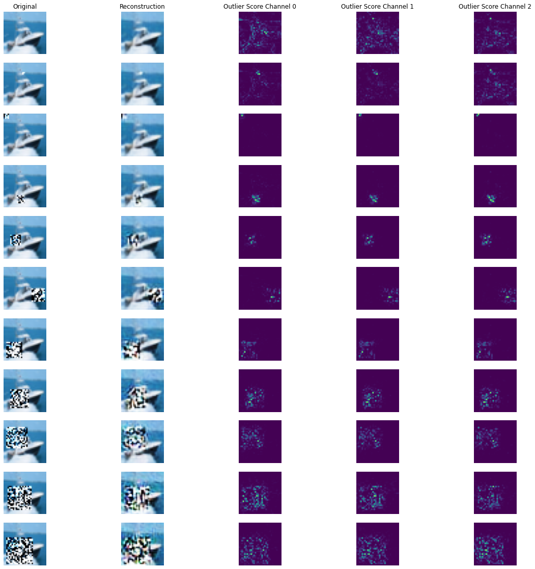
マスクされた画像の再構築とチャネル毎の外れ値スコア :
all_X_mask = []
X_i = X_orig[i].reshape(1, 32, 32, 3)
all_X_mask.append(X_i)
# apply masks
for j, mask_size in enumerate(mask_sizes):
    # create masked instances
    X_mask, mask = apply_mask(X_i,
                              mask_size=mask_size,
                              n_masks=1,  # just 1 for visualization purposes
                              channels=[0,1,2],
                              mask_type='normal',
                              noise_distr=(0,1),
                              clip_rng=(0,1))
    all_X_mask.append(X_mask)
all_X_mask = np.concatenate(all_X_mask, axis=0)
all_X_recon = od.vae(all_X_mask).numpy()
od_preds = od.predict(all_X_mask)
可視化します :
plot_feature_outlier_image(od_preds,
                           all_X_mask,
                           X_recon=all_X_recon,
                           max_instances=all_X_mask.shape[0],
                           n_channels=3)
(訳注 : 下は実験結果)
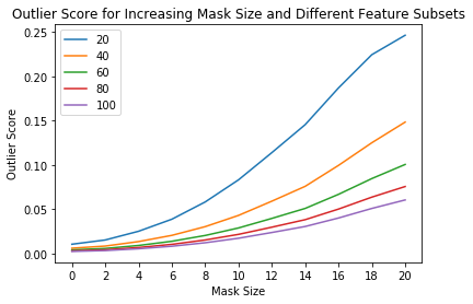
特徴のサブセットで外れ値を予測する
外れ値検知器の sensitivity (感度) は閾値を通してだけでなくインスタンスレベルの外れ値スコア計算のために使用される特徴のパーセンテージを選択することによっても制御できます。例えば、特徴の 40% が閾値を越える平均外れ値スコアを持つ場合外れ値であるとフラグ立てすることを望むかもしれません。これは predict 関数の outlier_perc 引数を通して可能です。それは降順の外れ値スコア順序でソートされた、外れ値検知のために使用される特徴のパーセンテージを指定します。
perc_list = [20, 40, 60, 80, 100]

all_perc_scores = []
for perc in perc_list:
    od_preds_perc = od.predict(all_X_mask, outlier_perc=perc)
    iscore = od_preds_perc['data']['instance_score']
    all_perc_scores.append(iscore)
外れ値スコア vs. マスクサイズと使用された特徴サイズのパーセンテージを可視化します :
x_plt = [0] + x_plt
for aps in all_perc_scores:
    plt.plot(x_plt, aps)
    plt.xticks(x_plt)
plt.legend(perc_list)
plt.title('Outlier Score for Increasing Mask Size and Different Feature Subsets')
plt.xlabel('Mask Size')
plt.ylabel('Outlier Score')
plt.show()
外れ値の閾値を推論する
良い閾値を見つけることは技巧的であり得ます、何故ならばそれらは典型的には解釈することが容易でないからです。infer_threshold メソッドは sensible な値を見つけるのに役立ちます。インスタンスのバッチ X を渡してそれらの何パーセントを正常であると考えるかを threshold_perc を通して指定する必要があります。
print('Current threshold: {}'.format(od.threshold))
od.infer_threshold(X, threshold_perc=99)  # assume 1% of the training data are outliers
print('New threshold: {}'.format(od.threshold))
Current threshold: 0.015
New threshold: 0.010383214280009267
(訳注 : 実験結果)
Current threshold: 0.015
New threshold: 0.0018019021837972088
以上
Alibi Detect 0.7 : Examples : AEGMM と VAEGMM 外れ値検知 on TCP dump
Alibi Detect 0.7 : Examples : AEGMM と VAEGMM 外れ値検知 on KDD Cup ‘99 データセット (翻訳/解説)
翻訳 : (株)クラスキャット セールスインフォメーション
作成日時 : 07/03/2021 (0.7.0)
* 本ページは、Alibi Detect の以下のドキュメントを翻訳した上で適宜、補足説明したものです:
- AEGMM and VAEGMM outlier detection on KDD Cup ‘99 dataset
- Auto-Encoding Gaussian Mixture Model
- Variational Auto-Encoding Gaussian Mixture Model
* サンプルコードの動作確認はしておりますが、必要な場合には適宜、追加改変しています。
* ご自由にリンクを張って頂いてかまいませんが、sales-info@classcat.com までご一報いただけると嬉しいです。
スケジュールは弊社 公式 Web サイト でご確認頂けます。
- お住まいの地域に関係なく Web ブラウザからご参加頂けます。事前登録 が必要ですのでご注意ください。
- ウェビナー運用には弊社製品「ClassCat® Webinar」を利用しています。
| 人工知能研究開発支援 | 人工知能研修サービス | テレワーク & オンライン授業を支援 |
| PoC(概念実証)を失敗させないための支援 (本支援はセミナーに参加しアンケートに回答した方を対象としています。) | ||
◆ お問合せ : 本件に関するお問い合わせ先は下記までお願いいたします。
| 株式会社クラスキャット セールス・マーケティング本部 セールス・インフォメーション |
| E-Mail:sales-info@classcat.com ; WebSite: https://www.classcat.com/ ; Facebook |
Alibi Detect 0.7 : Examples :AEGMM と VAEGMM 外れ値検知 on KDD Cup ‘99 データセット
AEGMM (オートエンコーディング・ガウス混合モデル) – 概要
オートエンコーディング・ガウス混合モデル (AEGMM) 外れ値検知器は 教師なし異常検知のための深層オートエンコーディング・ガウス混合モデル (Deep Autoencoding Gaussian Mixture Model for Unsupervised Anomaly Detection) 論文に従っています。エンコーダがデータを圧縮する一方で、デコーダにより生成された再構築されたインスタンスは入力と再構築の間の再構築誤差に基づいた追加の特徴を作成するために使用されます。これらの特徴はエンコーディングと結合されてガウス混合モデル (GMM) に供給されます。AEGMM 外れ値検知器はラベル付けされていない、しかし通常 (inlier) データのバッチ上で最初に訓練されます。教師なしか半教師あり訓練が望ましいです、何故ならばラベル付けされたデータはしばしば十分ではないからです。そして GMM のサンプルのエネルギーはインスタンスが外れ値 (高サンプル・エネルギー) か否か (低サンプル・エネルギー) を決定するために使用できます。このアルゴリズムは表形式か画像データのために適合します。
VAEGMM (変分オートエンコーディング・ガウス混合モデル) – 概要
変分オートエンコーディング・ガウス混合モデル (VAEGMM) 外れ値検知器は 教師なし異常検知のための深層オートエンコーディング・ガウス混合モデル (Deep Autoencoding Gaussian Mixture Model for Unsupervised Anomaly Detection) 論文に従っていますが、通常のオートエンコーダの代わりに VAE を使用します。エンコーダがデータを圧縮する一方で、デコーダにより生成された再構築されたインスタンスは入力と再構築の間の再構築誤差に基づいた追加の特徴を作成するために使用されます。これらの特徴はエンコーディングと結合されてガウス混合モデル (GMM) に供給されます。VAEGMM 外れ値検知器はラベル付けされていない、しかし通常 (inlier) データのバッチ上で最初に訓練されます。教師なしか半教師あり訓練が望ましいです、何故ならばラベル付けされたデータはしばしば十分ではないからです。そして GMM のサンプルのエネルギーはインスタンスが外れ値 (高サンプル・エネルギー) か否か (低サンプル・エネルギー) を決定するために使用できます。このアルゴリズムは表形式か画像データのために適合します。
データセット
典型的な U.S. 空軍 LAN をシミュレートした LAN の TCP dump データを使用して、外れ値検知器はコンピュータ・ネットワーク侵入を検知する必要があります。コネクションは明確に定義された時間で開始して終了する TCP パケットのシークエンスで、その間にデータは明確に定義されたプロトコルのもとにソース IP とターゲット IP アドレス間で流れます。各コネクションは正常、また攻撃としてラベル付けされます。
データセットには 4 タイプの攻撃があります :
- DOS: denial-of-service, e.g. syn flood;
- R2L: 遠隔マシンからの権限のないアクセス、e.g. パスワードの推測 ;
- U2R: ローカルのスーパーユーザ (root) 特権への権限のないアクセス ;
- probing : 偵察と他の厳密な調査、e.g., ポートスキャン。
データセットは約 500 万のコネクション・レコードを含みます。
3 つのタイプの特徴があります :
- 個々のコネクションの基本的な特徴, e.g. 接続時間 (duration of connection)
- コネクション内のコンテンツ特徴, e.g. 失敗したログイン試行の数
- 2 秒 window 内の traffic 特徴, e.g. 現在の接続と同じホストへのコネクションの数
import logging
import matplotlib.pyplot as plt
%matplotlib inline
import numpy as np
import pandas as pd
import seaborn as sns
from sklearn.metrics import confusion_matrix, f1_score
import tensorflow as tf
tf.keras.backend.clear_session()
from tensorflow.keras.layers import Dense, InputLayer

from alibi_detect.datasets import fetch_kdd
from alibi_detect.models.tensorflow.autoencoder import eucl_cosim_features
from alibi_detect.od import OutlierAEGMM, OutlierVAEGMM
from alibi_detect.utils.data import create_outlier_batch
from alibi_detect.utils.fetching import fetch_detector
from alibi_detect.utils.saving import save_detector, load_detector
from alibi_detect.utils.visualize import plot_instance_score, plot_feature_outlier_tabular, plot_roc

logger = tf.get_logger()
logger.setLevel(logging.ERROR)
データセットをロードする
幾つかの continuous (連続) な特徴 (41 の内から 18) だけを保持します。
kddcup = fetch_kdd(percent10=True)  # only load 10% of the dataset
print(kddcup.data.shape, kddcup.target.shape)
Downloading https://ndownloader.figshare.com/files/5976042
(494021, 18) (494021,)
kddcup.data[0]
array([8, 0.0, 0.0, 0.0, 0.0, 1.0, 0.0, 0.0, 9, 9, 1.0, 0.0, 0.11, 0.0,
       0.0, 0.0, 0.0, 0.0], dtype=object)
モデルはデータセットの (外れ値ではなく) 正常インスタンス上で訓練されて標準化 (= standardization) が適用されていると仮定します :
np.random.seed(0)
normal_batch = create_outlier_batch(kddcup.data, kddcup.target, n_samples=400000, perc_outlier=0)
X_train, y_train = normal_batch.data.astype('float32'), normal_batch.target
print(X_train.shape, y_train.shape)
print('{}% outliers'.format(100 * y_train.mean()))
(400000, 18) (400000,)
0.0% outliers
mean, stdev = X_train.mean(axis=0), X_train.std(axis=0)
print(mean)
print(stdev)
[1.09550075e+01 1.55620000e-03 1.74745000e-03 5.54626500e-02
 5.57733250e-02 9.85440925e-01 1.82663500e-02 1.33057100e-01
 1.48641492e+02 2.02133175e+02 8.44858050e-01 5.64032750e-02
 1.33479675e-01 2.40508250e-02 2.11637500e-03 1.05915000e-03
 5.73124750e-02 5.52324500e-02]
[2.17181039e+01 2.78305002e-02 2.61481724e-02 2.28073133e-01
 2.26952689e-01 9.25608777e-02 1.16637691e-01 2.77172101e-01
 1.03333220e+02 8.68577798e+01 3.05254458e-01 1.79868747e-01
 2.80221411e-01 4.92476707e-02 2.95181081e-02 1.59275611e-02
 2.24229381e-01 2.17798555e-01]
標準化を適用します :
X_train = (X_train - mean) / stdev
AEGMM 外れ値検知器をロードまたは定義する
examples ノートブックで使用される事前訓練済みの外れ値と敵対的検知器は ここ で見つかります。組込みの fetch_detector 関数を利用できます、これは事前訓練モデルをローカルディレクトリ filepath にセーブして検知器をロードします。代わりに、スクラッチから検知器を訓練することができます :
load_outlier_detector = False
filepath = 'model_aegmm' # 'my_path'  # change to directory (absolute path) where model is downloaded
if load_outlier_detector:  # load pretrained outlier detector
    detector_type = 'outlier'
    dataset = 'kddcup'
    detector_name = 'OutlierAEGMM'
    od = fetch_detector(filepath, detector_type, dataset, detector_name)
    filepath = os.path.join(filepath, detector_name)
else:  # define model, initialize, train and save outlier detector
    # the model defined here is similar to the one defined in the original paper
    n_features = X_train.shape[1]
    latent_dim = 1
    n_gmm = 2  # nb of components in GMM

    encoder_net = tf.keras.Sequential(
    [
        InputLayer(input_shape=(n_features,)),
        Dense(60, activation=tf.nn.tanh),
        Dense(30, activation=tf.nn.tanh),
        Dense(10, activation=tf.nn.tanh),
        Dense(latent_dim, activation=None)
    ])

    decoder_net = tf.keras.Sequential(
    [
        InputLayer(input_shape=(latent_dim,)),
        Dense(10, activation=tf.nn.tanh),
        Dense(30, activation=tf.nn.tanh),
        Dense(60, activation=tf.nn.tanh),
        Dense(n_features, activation=None)
    ])

    gmm_density_net = tf.keras.Sequential(
    [
        InputLayer(input_shape=(latent_dim + 2,)),
        Dense(10, activation=tf.nn.tanh),
        Dense(n_gmm, activation=tf.nn.softmax)
    ])

    # initialize outlier detector
    od = OutlierAEGMM(threshold=None,  # threshold for outlier score
                      encoder_net=encoder_net,         # can also pass AEGMM model instead
                      decoder_net=decoder_net,         # of separate encoder, decoder
                      gmm_density_net=gmm_density_net, # and gmm density net
                      n_gmm=n_gmm,
                      recon_features=eucl_cosim_features)  # fn used to derive features
                                                           # from the reconstructed
                                                           # instances based on cosine
                                                           # similarity and Eucl distance

    # train
    od.fit(X_train,
           epochs=50,
           batch_size=1024,
           #save_path=filepath,
           verbose=True)

    # save the trained outlier detector
    save_detector(od, filepath)
391/391 [=] - 10s 25ms/step - loss: 1.7450
391/391 [=] - 10s 26ms/step - loss: 1.6758
391/391 [=] - 10s 26ms/step - loss: 1.5309
391/391 [=] - 10s 25ms/step - loss: 1.4671
391/391 [=] - 10s 25ms/step - loss: 1.4172
391/391 [=] - 10s 25ms/step - loss: 1.3793
391/391 [=] - 10s 25ms/step - loss: 1.3396
391/391 [=] - 10s 26ms/step - loss: 1.2962
391/391 [=] - 10s 26ms/step - loss: 1.2483
391/391 [=] - 10s 25ms/step - loss: 1.2015
391/391 [=] - 10s 25ms/step - loss: 1.1678
391/391 [=] - 10s 25ms/step - loss: 1.1356
391/391 [=] - 10s 25ms/step - loss: 1.0989
391/391 [=] - 10s 26ms/step - loss: 1.0617
391/391 [=] - 10s 26ms/step - loss: 1.0288
391/391 [=] - 10s 25ms/step - loss: 0.9975
391/391 [=] - 10s 25ms/step - loss: 0.9630
391/391 [=] - 10s 25ms/step - loss: 0.9298
391/391 [=] - 10s 25ms/step - loss: 0.9013
391/391 [=] - 10s 26ms/step - loss: 0.8748
391/391 [=] - 11s 27ms/step - loss: 0.8481
391/391 [=] - 10s 25ms/step - loss: 0.8259
391/391 [=] - 10s 25ms/step - loss: 0.8081
391/391 [=] - 10s 25ms/step - loss: 0.7944
391/391 [=] - 10s 25ms/step - loss: 0.7825
391/391 [=] - 10s 26ms/step - loss: 0.7726
391/391 [=] - 10s 26ms/step - loss: 0.7628
391/391 [=] - 10s 25ms/step - loss: 0.7543
391/391 [=] - 10s 25ms/step - loss: 0.7460
391/391 [=] - 10s 25ms/step - loss: 0.7385
391/391 [=] - 10s 26ms/step - loss: 0.7314
391/391 [=] - 10s 26ms/step - loss: 0.7242
391/391 [=] - 10s 25ms/step - loss: 0.7185
391/391 [=] - 10s 25ms/step - loss: 0.7120
391/391 [=] - 10s 25ms/step - loss: 0.7064
391/391 [=] - 10s 25ms/step - loss: 0.7005
391/391 [=] - 10s 25ms/step - loss: 0.6947
391/391 [=] - 10s 26ms/step - loss: 0.6891
391/391 [=] - 11s 27ms/step - loss: 0.6844
391/391 [=] - 10s 25ms/step - loss: 0.6787
391/391 [=] - 10s 25ms/step - loss: 0.6738
391/391 [=] - 10s 25ms/step - loss: 0.6693
391/391 [=] - 10s 25ms/step - loss: 0.6648
391/391 [=] - 10s 26ms/step - loss: 0.6604
391/391 [=] - 10s 26ms/step - loss: 0.6561
391/391 [=] - 10s 25ms/step - loss: 0.6521
391/391 [=] - 10s 25ms/step - loss: 0.6476
391/391 [=] - 10s 25ms/step - loss: 0.6446
391/391 [=] - 10s 25ms/step - loss: 0.6409
391/391 [=] - 10s 26ms/step - loss: 0.6378
!ls model_aegmm -l
!ls model_aegmm/model -l
total 12
-rw-rw-r-- 1 ubuntu ubuntu  760  7月  3 07:33 OutlierAEGMM.pickle
-rw-rw-r-- 1 ubuntu ubuntu   89  7月  3 07:33 meta.pickle
drwxrwxr-x 2 ubuntu ubuntu 4096  7月  3 07:33 model
total 120
-rw-rw-r-- 1 ubuntu ubuntu 29329  7月  3 07:33 aegmm.ckpt.data-00000-of-00001
-rw-rw-r-- 1 ubuntu ubuntu  1398  7月  3 07:33 aegmm.ckpt.index
-rw-rw-r-- 1 ubuntu ubuntu    77  7月  3 07:33 checkpoint
-rw-rw-r-- 1 ubuntu ubuntu 31576  7月  3 07:33 decoder_net.h5
-rw-rw-r-- 1 ubuntu ubuntu 31608  7月  3 07:33 encoder_net.h5
-rw-rw-r-- 1 ubuntu ubuntu 14488  7月  3 07:33 gmm_density_net.h5
警告は outlier threshold (外れ値閾値) を依然として設定する必要があることを教えます。これは infer_threshold メソッドで成されます。インスタンスのバッチを渡してそれらの何パーセントを正常であると考えるかを threshold_perc を通して指定する必要があります。およそ 5% の外れ値を含むことを知るあるデータを持つと仮定しましょう。外れ値のパーセンテージは create_outlier_batch 関数で perc_outlier で設定できます。
np.random.seed(0)
perc_outlier = 5
threshold_batch = create_outlier_batch(kddcup.data, kddcup.target, n_samples=1000, perc_outlier=perc_outlier)
X_threshold, y_threshold = threshold_batch.data.astype('float32'), threshold_batch.target
X_threshold = (X_threshold - mean) / stdev
print('{}% outliers'.format(100 * y_threshold.mean()))
5.0% outliers
od.infer_threshold(X_threshold, threshold_perc=100-perc_outlier)
print('New threshold: {}'.format(od.threshold))
New threshold: 5.188828468322754
更新された閾値で外れ値検知器をセーブしましょう :
save_detector(od, filepath)
外れ値を検出する
今は 10% の外れ値を持つデータのバッチを生成しそしてバッチ内の外れ値を検出します。
np.random.seed(1)
outlier_batch = create_outlier_batch(kddcup.data, kddcup.target, n_samples=1000, perc_outlier=10)
X_outlier, y_outlier = outlier_batch.data.astype('float32'), outlier_batch.target
X_outlier = (X_outlier - mean) / stdev
print(X_outlier.shape, y_outlier.shape)
print('{}% outliers'.format(100 * y_outlier.mean()))
(1000, 18) (1000,)
10.0% outliers
外れ値を予測します :
od_preds = od.predict(X_outlier, return_instance_score=True)
結果を表示する
F1 スコアと混同行列 :
labels = outlier_batch.target_names
y_pred = od_preds['data']['is_outlier']
f1 = f1_score(y_outlier, y_pred)
print('F1 score: {:.4f}'.format(f1))
cm = confusion_matrix(y_outlier, y_pred)
df_cm = pd.DataFrame(cm, index=labels, columns=labels)
sns.heatmap(df_cm, annot=True, cbar=True, linewidths=.5)
plt.show()
F1 score: 0.3352
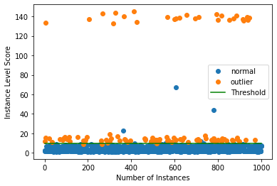
インスタンスレベルの外れ値スコア vs 外れ値閾値をプロットします :
plot_instance_score(od_preds, y_outlier, labels, od.threshold, ylim=(None, None))
検出器の外れ値スコアのための ROC カーブをプロットすることもできます :
roc_data = {'AEGMM': {'scores': od_preds['data']['instance_score'], 'labels': y_outlier}}
plot_roc(roc_data)
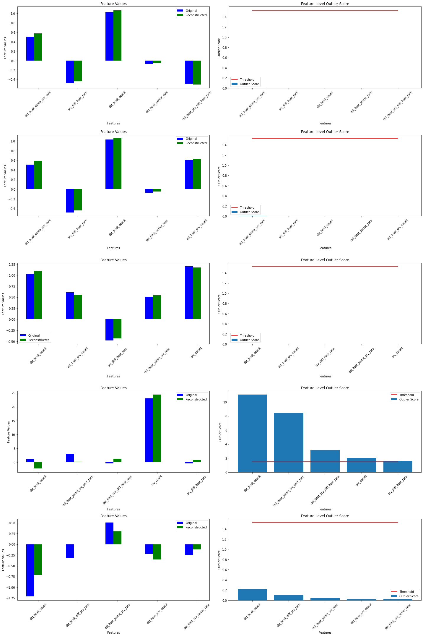
インスタンスレベル外れ値を調査する
潜在空間のインスタンスのエンコーディングとデコーダにより再構築されたインスタンスに由来する特徴を可視化できます。そしてエンコーディングと特徴は GMM 密度ネットワークに供給されます。
enc = od.aegmm.encoder(X_outlier)  # encoding
X_recon = od.aegmm.decoder(enc)  # reconstructed instances
recon_features = od.aegmm.recon_features(X_outlier, X_recon)  # reconstructed features
df = pd.DataFrame(dict(enc=enc[:, 0].numpy(),
                       cos=recon_features[:, 0].numpy(),
                       eucl=recon_features[:, 1].numpy(),
                       label=y_outlier))

groups = df.groupby('label')
fig, ax = plt.subplots()
for name, group in groups:
    ax.plot(group.enc, group.cos, marker='o',
            linestyle='', ms=6, label=labels[name])
plt.title('Encoding vs. Cosine Similarity')
plt.xlabel('Encoding')
plt.ylabel('Cosine Similarity')
ax.legend()
plt.show()

fig, ax = plt.subplots()
for name, group in groups:
    ax.plot(group.enc, group.eucl, marker='o',
            linestyle='', ms=6, label=labels[name])
plt.title('Encoding vs. Relative Euclidean Distance')
plt.xlabel('Encoding')
plt.ylabel('Relative Euclidean Distance')
ax.legend()
plt.show()
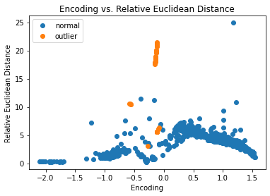
多くの外れ値が潜在空間で既に上手く分離されています。
VAEGMM 外れ値検知器を使用する
Google Cloud Bucket から 事前訓練済みの VAEGMM 検出器を再度インスタンス化できます。組込みの fetch_detector 関数を利用できます、これは事前訓練モデルをローカルディレクトリ filepath にセーブして検知器をロードします。代わりに、スクラッチから検知器を訓練することができます :
load_outlier_detector = False
filepath = 'model_vaegmm'  # change to directory (absolute path) where model is downloaded
if load_outlier_detector:  # load pretrained outlier detector
    detector_type = 'outlier'
    dataset = 'kddcup'
    detector_name = 'OutlierVAEGMM'
    od = fetch_detector(filepath, detector_type, dataset, detector_name)
    filepath = os.path.join(filepath, detector_name)
else:  # define model, initialize, train and save outlier detector
    # the model defined here is similar to the one defined in
    # the OutlierVAE notebook
    n_features = X_train.shape[1]
    latent_dim = 2
    n_gmm = 2

    encoder_net = tf.keras.Sequential(
    [
        InputLayer(input_shape=(n_features,)),
        Dense(20, activation=tf.nn.relu),
        Dense(15, activation=tf.nn.relu),
        Dense(7, activation=tf.nn.relu)
    ])

    decoder_net = tf.keras.Sequential(
    [
        InputLayer(input_shape=(latent_dim,)),
        Dense(7, activation=tf.nn.relu),
        Dense(15, activation=tf.nn.relu),
        Dense(20, activation=tf.nn.relu),
        Dense(n_features, activation=None)
    ])

    gmm_density_net = tf.keras.Sequential(
    [
        InputLayer(input_shape=(latent_dim + 2,)),
        Dense(10, activation=tf.nn.relu),
        Dense(n_gmm, activation=tf.nn.softmax)
    ])


    # initialize outlier detector
    od = OutlierVAEGMM(threshold=None,
                       encoder_net=encoder_net,
                       decoder_net=decoder_net,
                       gmm_density_net=gmm_density_net,
                       n_gmm=n_gmm,
                       latent_dim=latent_dim,
                       samples=10,
                       recon_features=eucl_cosim_features)

    # train
    od.fit(X_train,
           epochs=50,
           batch_size=1024,
           cov_elbo=dict(sim=.0025),  # standard deviation assumption
           verbose=True)           # for elbo training

    # save the trained outlier detector
    save_detector(od, filepath)
391/391 [=] - 16s 40ms/step - loss: 0.7435
391/391 [=] - 15s 39ms/step - loss: 0.6727
391/391 [=] - 15s 38ms/step - loss: 0.6538
391/391 [=] - 15s 38ms/step - loss: 0.6449
391/391 [=] - 16s 40ms/step - loss: 0.6384
391/391 [=] - 15s 38ms/step - loss: 0.6383
391/391 [=] - 15s 38ms/step - loss: 0.6410
391/391 [=] - 16s 40ms/step - loss: 0.6557
391/391 [=] - 15s 39ms/step - loss: 0.7462
391/391 [=] - 15s 38ms/step - loss: 0.9006
391/391 [=] - 15s 38ms/step - loss: 0.8419
391/391 [=] - 15s 39ms/step - loss: 0.8301
391/391 [=] - 16s 41ms/step - loss: 0.8225
391/391 [=] - 15s 38ms/step - loss: 0.8158
391/391 [=] - 15s 39ms/step - loss: 0.8086
391/391 [=] - 15s 39ms/step - loss: 0.8014
391/391 [=] - 16s 40ms/step - loss: 0.7956
391/391 [=] - 15s 39ms/step - loss: 0.7901
391/391 [=] - 15s 39ms/step - loss: 0.7835
391/391 [=] - 15s 39ms/step - loss: 0.7772
391/391 [=] - 15s 39ms/step - loss: 0.7687
391/391 [=] - 15s 39ms/step - loss: 0.7593
391/391 [=] - 15s 39ms/step - loss: 0.7490
391/391 [=] - 15s 39ms/step - loss: 0.7400
391/391 [=] - 16s 41ms/step - loss: 0.7326
391/391 [=] - 15s 39ms/step - loss: 0.7261
391/391 [=] - 15s 39ms/step - loss: 0.7212
391/391 [=] - 16s 40ms/step - loss: 0.7167
391/391 [=] - 16s 40ms/step - loss: 0.7125
391/391 [=] - 15s 39ms/step - loss: 0.7068
391/391 [=] - 15s 39ms/step - loss: 0.7023
391/391 [=] - 16s 40ms/step - loss: 0.6979
391/391 [=] - 15s 39ms/step - loss: 0.6941
391/391 [=] - 15s 39ms/step - loss: 0.6903
391/391 [=] - 15s 39ms/step - loss: 0.6883
391/391 [=] - 16s 40ms/step - loss: 0.6861
391/391 [=] - 16s 40ms/step - loss: 0.6843
391/391 [=] - 15s 39ms/step - loss: 0.6829
391/391 [=] - 15s 39ms/step - loss: 0.6814
391/391 [=] - 16s 41ms/step - loss: 0.6802
391/391 [=] - 15s 39ms/step - loss: 0.6791
391/391 [=] - 15s 39ms/step - loss: 0.6786
391/391 [=] - 15s 39ms/step - loss: 0.6774
391/391 [=] - 16s 40ms/step - loss: 0.6767
391/391 [=] - 15s 39ms/step - loss: 0.6759
391/391 [=] - 15s 39ms/step - loss: 0.6756
391/391 [=] - 15s 40ms/step - loss: 0.6753
391/391 [=] - 16s 41ms/step - loss: 0.6741
391/391 [=] - 15s 39ms/step - loss: 0.6729
391/391 [=] - 15s 39ms/step - loss: 0.6733
!ls model_vaegmm -l
!ls model_vaegmm/model -l
total 12
-rw-rw-r-- 1 ubuntu ubuntu  935  7月  3 07:56 OutlierVAEGMM.pickle
-rw-rw-r-- 1 ubuntu ubuntu   90  7月  3 07:56 meta.pickle
drwxrwxr-x 2 ubuntu ubuntu 4096  7月  3 07:56 model
total 80
-rw-rw-r-- 1 ubuntu ubuntu    79  7月  3 07:56 checkpoint
-rw-rw-r-- 1 ubuntu ubuntu 22104  7月  3 07:56 decoder_net.h5
-rw-rw-r-- 1 ubuntu ubuntu 19304  7月  3 07:56 encoder_net.h5
-rw-rw-r-- 1 ubuntu ubuntu 14488  7月  3 07:56 gmm_density_net.h5
-rw-rw-r-- 1 ubuntu ubuntu 10033  7月  3 07:56 vaegmm.ckpt.data-00000-of-00001
-rw-rw-r-- 1 ubuntu ubuntu  1503  7月  3 07:56 vaegmm.ckpt.index
再度閾値を推論する必要があります :
od.infer_threshold(X_threshold, threshold_perc=100-perc_outlier)
print('New threshold: {}'.format(od.threshold))
New threshold: 9.472237873077368
更新された閾値で外れ値検知器をセーブします :
save_detector(od, filepath)
外れ値を検出して結果を表示する
予測します :
od_preds = od.predict(X_outlier, return_instance_score=True)
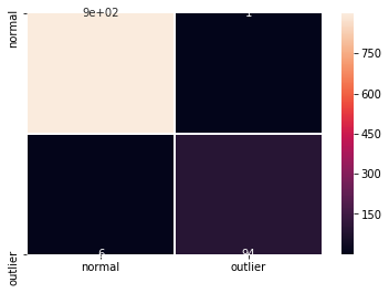
F1 スコアと混同行列 :
labels = outlier_batch.target_names
y_pred = od_preds['data']['is_outlier']
f1 = f1_score(y_outlier, y_pred)
print('F1 score: {:.4f}'.format(f1))
cm = confusion_matrix(y_outlier, y_pred)
df_cm = pd.DataFrame(cm, index=labels, columns=labels)
sns.heatmap(df_cm, annot=True, cbar=True, linewidths=.5)
plt.show()
F1 score: 0.9515

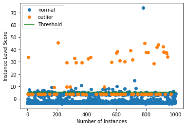
インスタンスレベルの外れ値スコア vs 外れ値閾値をプロットします :
plot_instance_score(od_preds, y_outlier, labels, od.threshold, ylim=(None, None))
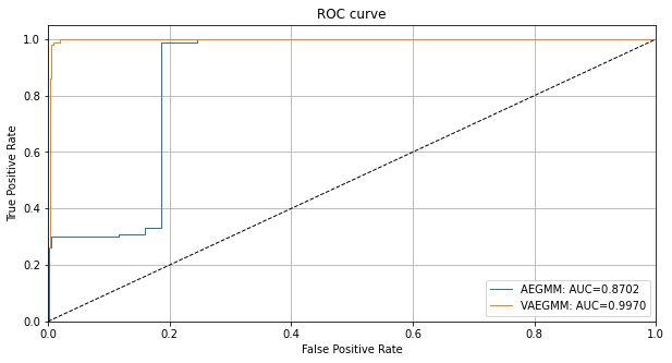
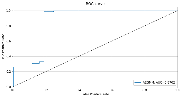
ylim の min と max 値を調整することによりズームインできます。VAEGMM ROC カーブを AEGMM と比較することもできます :
roc_data['VAEGMM'] = {'scores': od_preds['data']['instance_score'], 'labels': y_outlier}
plot_roc(roc_data)
以上
Alibi Detect 0.7 : Examples : VAE 外れ値検知 on TCP dump
Alibi Detect 0.7 : Examples : VAE 外れ値検知 on KDD Cup ‘99 データセット (翻訳/解説)
翻訳 : (株)クラスキャット セールスインフォメーション
作成日時 : 07/02/2021 (0.7.0)
* 本ページは、Alibi Detect の以下のドキュメントを翻訳した上で適宜、補足説明したものです:
* サンプルコードの動作確認はしておりますが、必要な場合には適宜、追加改変しています。
* ご自由にリンクを張って頂いてかまいませんが、sales-info@classcat.com までご一報いただけると嬉しいです。
スケジュールは弊社 公式 Web サイト でご確認頂けます。
- お住まいの地域に関係なく Web ブラウザからご参加頂けます。事前登録 が必要ですのでご注意ください。
- ウェビナー運用には弊社製品「ClassCat® Webinar」を利用しています。
| 人工知能研究開発支援 | 人工知能研修サービス | テレワーク & オンライン授業を支援 |
| PoC(概念実証)を失敗させないための支援 (本支援はセミナーに参加しアンケートに回答した方を対象としています。) | ||
◆ お問合せ : 本件に関するお問い合わせ先は下記までお願いいたします。
| 株式会社クラスキャット セールス・マーケティング本部 セールス・インフォメーション |
| E-Mail:sales-info@classcat.com ; WebSite: https://www.classcat.com/ ; Facebook |
Alibi Detect 0.7 : Examples : VAE 外れ値検知 on KDD Cup ‘99 データセット
VAE – 概要
変分オートエンコーダ (VAE, Variational Auto-Encoder) 外れ値検知器は最初にラベル付けされていない、しかし通常 (inlier) データのバッチで訓練されます。教師なしか半教師あり訓練が望ましいです、何故ならばラベル付けされたデータはしばしば十分でないからです。VAE 検知器はそれが受け取る入力を再構築しようとします。入力データが上手く再構築されない場合、再構築エラーは高くそしてデータは外れ値としてフラグ立てできます。再構築エラーは、入力と再構築されたインスタンスの間の平均二乗誤差 (MSE, mean squared error) か、入力と再構築されたインスタンスの両者が同じプロセスで生成される確率として測定されます。アルゴリズムは表形式か画像データのために適合します。
データセット
典型的な U.S. 空軍 LAN をシミュレートした LAN の TCP dump データを使用して、外れ値検知器はコンピュータ・ネットワーク侵入を検知する必要があります。コネクションは明確に定義された時間で開始して終了する TCP パケットのシークエンスで、その間にデータは明確に定義されたプロトコルのもとにソース IP とターゲット IP アドレス間で流れます。各コネクションは正常、また攻撃としてラベル付けされます。
データセットには 4 タイプの攻撃があります :
- DOS: denial-of-service, e.g. syn flood;
- R2L: 遠隔マシンからの権限のないアクセス、e.g. パスワードの推測 ;
- U2R: ローカルのスーパーユーザ (root) 特権への権限のないアクセス ;
- probing : 偵察と他の厳密な調査、e.g., ポートスキャン。
データセットは約 500 万のコネクション・レコードを含みます。
3 つのタイプの特徴があります :
- 個々のコネクションの基本的な特徴, e.g. 接続時間 (duration of connection)
- コネクション内のコンテンツ特徴, e.g. 失敗したログイン試行の数
- 2 秒 window 内の traffic 特徴, e.g. 現在の接続と同じホストへのコネクションの数
import logging
import matplotlib.pyplot as plt
%matplotlib inline
import numpy as np
import pandas as pd
import seaborn as sns
from sklearn.metrics import confusion_matrix, f1_score
import tensorflow as tf
tf.keras.backend.clear_session()
from tensorflow.keras.layers import Dense, InputLayer

from alibi_detect.datasets import fetch_kdd
from alibi_detect.models.tensorflow.losses import elbo
from alibi_detect.od import OutlierVAE
from alibi_detect.utils.data import create_outlier_batch
from alibi_detect.utils.fetching import fetch_detector
from alibi_detect.utils.saving import save_detector, load_detector
from alibi_detect.utils.visualize import plot_instance_score, plot_feature_outlier_tabular, plot_roc

logger = tf.get_logger()
logger.setLevel(logging.ERROR)
データセットをロードする
幾つかの continuous (連続) な特徴 (41 の内から 18) だけを保持します。
kddcup = fetch_kdd(percent10=True)  # only load 10% of the dataset
print(kddcup.data.shape, kddcup.target.shape)
Downloading https://ndownloader.figshare.com/files/5976042
(494021, 18) (494021,)
kddcup.data[0]
array([8, 0.0, 0.0, 0.0, 0.0, 1.0, 0.0, 0.0, 9, 9, 1.0, 0.0, 0.11, 0.0,
       0.0, 0.0, 0.0, 0.0], dtype=object)
機械学習モデルはデータセットの (外れ値ではなく) 正常インスタンス上で訓練されて標準化 (= standardization) が適用されていると仮定します :
np.random.seed(0)
normal_batch = create_outlier_batch(kddcup.data, kddcup.target, n_samples=400000, perc_outlier=0)
X_train, y_train = normal_batch.data.astype('float'), normal_batch.target
print(X_train.shape, y_train.shape)
print('{}% outliers'.format(100 * y_train.mean()))
(400000, 18) (400000,)
0.0% outliers
mean, stdev = X_train.mean(axis=0), X_train.std(axis=0)
print(mean)
print(stdev)
[1.09550075e+01 1.55620000e-03 1.74745000e-03 5.54626500e-02
 5.57733250e-02 9.85440925e-01 1.82663500e-02 1.33057100e-01
 1.48641492e+02 2.02133175e+02 8.44858050e-01 5.64032750e-02
 1.33479675e-01 2.40508250e-02 2.11637500e-03 1.05915000e-03
 5.73124750e-02 5.52324500e-02]
[2.17181039e+01 2.78305002e-02 2.61481724e-02 2.28073133e-01
 2.26952689e-01 9.25608777e-02 1.16637691e-01 2.77172101e-01
 1.03333220e+02 8.68577798e+01 3.05254458e-01 1.79868747e-01
 2.80221411e-01 4.92476707e-02 2.95181081e-02 1.59275611e-02
 2.24229381e-01 2.17798555e-01]
標準化を適用します :
X_train = (X_train - mean) / stdev
外れ値検知器をロードまたは定義する
examples ノートブックで使用される事前訓練済みの外れ値と敵対的検知器は ここ で見つかります。組込みの fetch_detector 関数を利用できます、これは事前訓練モデルをローカルディレクトリ filepath にセーブして検知器をロードします。代わりに、スクラッチから検知器を訓練することができます。
load_outlier_detector = False
filepath = 'my_dir'  # change to directory (absolute path) where model is downloaded
if load_outlier_detector:  # load pretrained outlier detector
    detector_type = 'outlier'
    dataset = 'kddcup'
    detector_name = 'OutlierVAE'
    od = fetch_detector(filepath, detector_type, dataset, detector_name)
    filepath = os.path.join(filepath, detector_name)
else:  # define model, initialize, train and save outlier detector
    n_features = X_train.shape[1]
    latent_dim = 2

    encoder_net = tf.keras.Sequential(
      [
          InputLayer(input_shape=(n_features,)),
          Dense(20, activation=tf.nn.relu),
          Dense(15, activation=tf.nn.relu),
          Dense(7, activation=tf.nn.relu)
      ])

    decoder_net = tf.keras.Sequential(
      [
          InputLayer(input_shape=(latent_dim,)),
          Dense(7, activation=tf.nn.relu),
          Dense(15, activation=tf.nn.relu),
          Dense(20, activation=tf.nn.relu),
          Dense(n_features, activation=None)
      ])

    # initialize outlier detector
    od = OutlierVAE(threshold=None,  # threshold for outlier score
                    score_type='mse',  # use MSE of reconstruction error for outlier detection
                    encoder_net=encoder_net,  # can also pass VAE model instead
                    decoder_net=decoder_net,  # of separate encoder and decoder
                    latent_dim=latent_dim,
                    samples=5)
    # train
    od.fit(X_train,
           loss_fn=elbo,
           cov_elbo=dict(sim=.01),
           epochs=30,
           verbose=True)

    # save the trained outlier detector
    save_detector(od, filepath)
6250/6250 [=] - 148s 24ms/step - loss: 28695.7242
6250/6250 [=] - 148s 24ms/step - loss: 12437.6854
6250/6250 [=] - 146s 23ms/step - loss: 10256.9219
6250/6250 [=] - 155s 25ms/step - loss: 9557.9839
6250/6250 [=] - 147s 23ms/step - loss: 8414.8731
6250/6250 [=] - 148s 24ms/step - loss: 7847.7130
6250/6250 [=] - 151s 24ms/step - loss: 7549.5546
6250/6250 [=] - 150s 24ms/step - loss: 7412.6179
6250/6250 [=] - 147s 23ms/step - loss: 7358.9181
6250/6250 [=] - 148s 24ms/step - loss: 7064.3351
6250/6250 [=] - 145s 23ms/step - loss: 7047.5733
6250/6250 [=] - 150s 24ms/step - loss: 6862.8724
6250/6250 [=] - 146s 23ms/step - loss: 6859.6950
6250/6250 [=] - 149s 24ms/step - loss: 6733.0950
6250/6250 [=] - 146s 23ms/step - loss: 6395.8519
6250/6250 [=] - 152s 24ms/step - loss: 6239.8235
6250/6250 [=] - 147s 23ms/step - loss: 6141.0218
6250/6250 [=] - 149s 24ms/step - loss: 6080.4994
6250/6250 [=] - 150s 24ms/step - loss: 6030.9626
6250/6250 [=] - 152s 24ms/step - loss: 5986.5710
6250/6250 [=] - 152s 24ms/step - loss: 5968.1871
6250/6250 [=] - 150s 24ms/step - loss: 6026.3471
6250/6250 [=] - 152s 24ms/step - loss: 5828.1424
6250/6250 [=] - 149s 24ms/step - loss: 5841.5844
6250/6250 [=] - 147s 24ms/step - loss: 5794.9508
6250/6250 [=] - 154s 25ms/step - loss: 5792.5575
6250/6250 [=] - 147s 24ms/step - loss: 5767.5592
6250/6250 [=] - 150s 24ms/step - loss: 5643.3078
6250/6250 [=] - 147s 23ms/step - loss: 5571.4557
6250/6250 [=] - 148s 24ms/step - loss: 5541.4037
!ls model_vae -l
!ls model_vae/model -l
total 12
-rw-rw-r-- 1 ubuntu ubuntu  107  7月  2 13:26 OutlierVAE.pickle
-rw-rw-r-- 1 ubuntu ubuntu   87  7月  2 13:26 meta.pickle
drwxrwxr-x 2 ubuntu ubuntu 4096  7月  2 13:26 model
total 64
-rw-rw-r-- 1 ubuntu ubuntu    73  7月  2 13:26 checkpoint
-rw-rw-r-- 1 ubuntu ubuntu 22104  7月  2 13:26 decoder_net.h5
-rw-rw-r-- 1 ubuntu ubuntu 19304  7月  2 13:26 encoder_net.h5
-rw-rw-r-- 1 ubuntu ubuntu  9269  7月  2 13:26 vae.ckpt.data-00000-of-00001
-rw-rw-r-- 1 ubuntu ubuntu  1259  7月  2 13:26 vae.ckpt.index
警告は outlier threshold (外れ値閾値) を依然として設定する必要があることを教えます。これは infer_threshold メソッドで成されます。インスタンスのバッチを渡してそれらの何パーセントを正常であると考えるかを threshold_perc を通して指定する必要があります。およそ 5% の外れ値を含むことを知るあるデータを持つと仮定しましょう。外れ値のパーセンテージは create_outlier_batch 関数で perc_outlier で設定できます。
np.random.seed(0)
perc_outlier = 5
threshold_batch = create_outlier_batch(kddcup.data, kddcup.target, n_samples=1000, perc_outlier=perc_outlier)
X_threshold, y_threshold = threshold_batch.data.astype('float'), threshold_batch.target
X_threshold = (X_threshold - mean) / stdev
print('{}% outliers'.format(100 * y_threshold.mean()))
5.0% outliers
od.infer_threshold(X_threshold, threshold_perc=100-perc_outlier)
print('New threshold: {}'.format(od.threshold))
New threshold: 1.5222603200798008
threshold_perc を例えば 99 に設定して推論された閾値に少しのマージンを加えることにより通常の訓練データから閾値をすいろんすることもできました。更新された閾値で外れ値検知器をセーブしましょう :
save_detector(od, filepath)
!ls model_vae -l
!ls model_vae/model -l
total 12
-rw-rw-r-- 1 ubuntu ubuntu  218  7月  2 13:35 OutlierVAE.pickle
-rw-rw-r-- 1 ubuntu ubuntu   87  7月  2 13:35 meta.pickle
drwxrwxr-x 2 ubuntu ubuntu 4096  7月  2 13:35 model
total 64
-rw-rw-r-- 1 ubuntu ubuntu    73  7月  2 13:35 checkpoint
-rw-rw-r-- 1 ubuntu ubuntu 22104  7月  2 13:35 decoder_net.h5
-rw-rw-r-- 1 ubuntu ubuntu 19304  7月  2 13:35 encoder_net.h5
-rw-rw-r-- 1 ubuntu ubuntu  9269  7月  2 13:35 vae.ckpt.data-00000-of-00001
-rw-rw-r-- 1 ubuntu ubuntu  1259  7月  2 13:35 vae.ckpt.index
外れ値を検出する
今は 10% の外れ値を持つデータのバッチを生成しそしてバッチ内の外れ値を検出します。
np.random.seed(1)
outlier_batch = create_outlier_batch(kddcup.data, kddcup.target, n_samples=1000, perc_outlier=10)
X_outlier, y_outlier = outlier_batch.data.astype('float'), outlier_batch.target
X_outlier = (X_outlier - mean) / stdev
print(X_outlier.shape, y_outlier.shape)
print('{}% outliers'.format(100 * y_outlier.mean()))
(1000, 18) (1000,)
10.0% outliers
外れ値を予測します :
od_preds = od.predict(X_outlier,
                      outlier_type='instance',    # use 'feature' or 'instance' level
                      return_feature_score=True,  # scores used to determine outliers
                      return_instance_score=True)
print(list(od_preds['data'].keys()))
['instance_score', 'feature_score', 'is_outlier']
od_preds['data']['is_outlier'][:10]
array([0, 0, 0, 1, 0, 1, 1, 0, 0, 0])
od_preds['data']['instance_score'][:10]
array([5.74442137e-04, 6.24835379e-04, 6.83877481e-04, 1.52228703e+00,
       2.47923307e-02, 4.29582862e+01, 1.52229905e+00, 4.45219175e-03,
       8.09561496e-02, 2.37765956e-02])
od_preds['data']['feature_score']
array([[4.77347707e-05, 6.23364775e-05, 4.80892692e-05, ...,
        3.21192958e-04, 6.79559419e-05, 5.60611257e-05],
       [1.67435697e-04, 7.68863402e-05, 1.12371712e-04, ...,
        3.19287128e-04, 9.01695907e-05, 8.10840695e-05],
       [9.42410698e-04, 1.08231414e-06, 3.40019366e-05, ...,
        5.65485925e-04, 1.88107799e-05, 1.04572967e-05],
       ...,
       [2.08158688e-03, 4.93670543e-06, 3.57241685e-05, ...,
        6.89739720e-04, 9.91289453e-05, 3.80882650e-06],
       [2.27466705e-03, 4.25181944e-03, 6.06307292e-05, ...,
        3.40673684e-05, 9.27018184e-06, 6.57232246e-03],
       [1.50122506e-03, 4.51257037e-03, 1.09080541e-05, ...,
        4.76422446e-04, 4.67411636e-03, 4.86378648e-02]])
結果を表示する
F1 スコアと混同行列 :
labels = outlier_batch.target_names
y_pred = od_preds['data']['is_outlier']
f1 = f1_score(y_outlier, y_pred)
print('F1 score: {:.4f}'.format(f1))
cm = confusion_matrix(y_outlier, y_pred)
df_cm = pd.DataFrame(cm, index=labels, columns=labels)
sns.heatmap(df_cm, annot=True, cbar=True, linewidths=.5)
plt.show()
F1 score: 0.9754
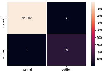
インスタンスレベルの外れ値スコア vs 外れ値閾値をプロットします :
plot_instance_score(od_preds, y_outlier, labels, od.threshold)
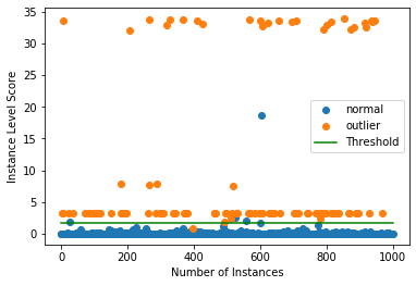
幾つかの外れ値が検出するのに非常に簡単である一方で、他は通常データに近い外れ値スコアを持つことが明瞭に分かります。検出器の外れ値スコアのための ROC カーブをプロットすることもできます :
roc_data = {'VAE': {'scores': od_preds['data']['instance_score'], 'labels': y_outlier}}
plot_roc(roc_data)
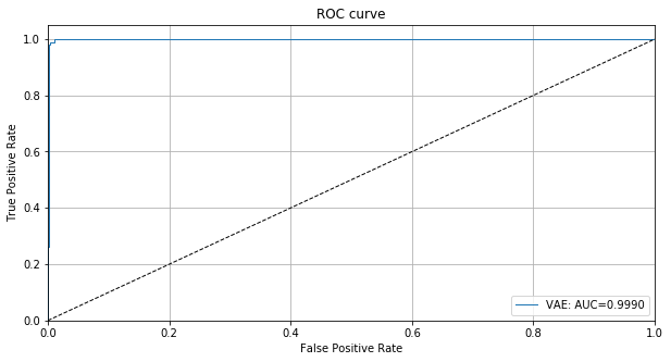
インスタンスレベル外れ値を調査する
今は X_outlier 上の個々の予測の幾つかを詳しく見ることができます。
X_recon = od.vae(X_outlier).numpy() # reconstructed instances by the VAE
plot_feature_outlier_tabular(od_preds,
                             X_outlier,
                             X_recon=X_recon,
                             threshold=od.threshold,
                             instance_ids=None,  # pass a list with indices of instances to display
                             max_instances=5,  # max nb of instances to display
                             top_n=5,  # only show top_n features ordered by outlier score
                             outliers_only=False,  # only show outlier predictions
                             feature_names=kddcup.feature_names,  # add feature names
                             figsize=(20, 30))
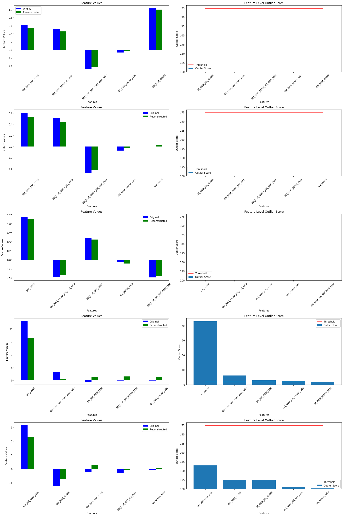
(訳注 : 下は実験結果)
srv_count 特徴は多くの表示される外れ値の責任を負います。
以上
Alibi Detect 0.7 : Examples : Isolation Forest 外れ値検知 on TCP dump
Alibi Detect 0.7 : Examples : Isolation Forest 外れ値検知 on KDD Cup ‘99 データセット (翻訳/解説)
翻訳 : (株)クラスキャット セールスインフォメーション
作成日時 : 07/02/2021 (0.7.0)
* 本ページは、Alibi Detect の以下のドキュメントを翻訳した上で適宜、補足説明したものです:
* サンプルコードの動作確認はしておりますが、必要な場合には適宜、追加改変しています。
* ご自由にリンクを張って頂いてかまいませんが、sales-info@classcat.com までご一報いただけると嬉しいです。
スケジュールは弊社 公式 Web サイト でご確認頂けます。
- お住まいの地域に関係なく Web ブラウザからご参加頂けます。事前登録 が必要ですのでご注意ください。
- ウェビナー運用には弊社製品「ClassCat® Webinar」を利用しています。
| 人工知能研究開発支援 | 人工知能研修サービス | テレワーク & オンライン授業を支援 |
| PoC(概念実証)を失敗させないための支援 (本支援はセミナーに参加しアンケートに回答した方を対象としています。) | ||
◆ お問合せ : 本件に関するお問い合わせ先は下記までお願いいたします。
| 株式会社クラスキャット セールス・マーケティング本部 セールス・インフォメーション |
| E-Mail:sales-info@classcat.com ; WebSite: https://www.classcat.com/ ; Facebook |
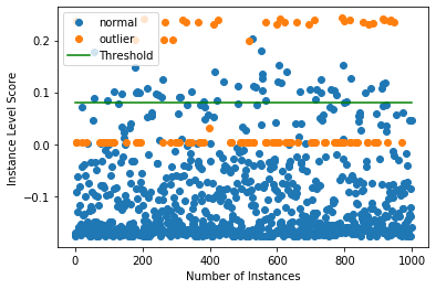
Alibi Detect 0.7 : Examples : Isolation Forest 外れ値検知 on KDD Cup ‘99 データセット
Isolation Forest – 概要
Isolation forests (IF) は特に外れ値検知のために使用される tree ベースのモデルです。IF は特徴をランダムに選択してから選択された特徴の最大値と最小値の間の分割値をランダムに選択することにより観測を isolate (分離、区分け) します。サンプルを区分けするために必要な分割の数はルートノードから終端 (= terminating) ノードへのパスの長さに等しいです。ランダム tree の森に渡り平均された、パスの長さは正常の尺度で異常スコアを定義するために使用されます。外れ値は典型的にはより迅速に分離され、より短いパスに繋がります。アルゴリズムは低次元から medium 次元の表形式データのために適します。
データセット
典型的な U.S. 空軍 LAN をシミュレートした LAN の TCP dump データを使用して、外れ値検知器はコンピュータ・ネットワーク侵入を検知する必要があります。コネクションは明確に定義された時間で開始して終了する TCP パケットのシークエンスで、その間にデータは明確に定義されたプロトコルのもとにソース IP とターゲット IP アドレス間で流れます。各コネクションは正常、また攻撃としてラベル付けされます。
データセットには 4 タイプの攻撃があります :
- DOS: denial-of-service, e.g. syn flood;
- R2L: 遠隔マシンからの権限のないアクセス、e.g. パスワードの推測 ;
- U2R: ローカルのスーパーユーザ (root) 特権への権限のないアクセス ;
- probing : 偵察と他の厳密な調査、e.g., ポートスキャン。
データセットは約 500 万のコネクション・レコードを含みます。
3 つのタイプの特徴があります :
- 個々のコネクションの基本的な特徴, e.g. 接続時間 (duration of connection)
- コネクション内のコンテンツ特徴, e.g. 失敗したログイン試行の数
- 2 秒 window 内の traffic 特徴, e.g. 現在の接続と同じホストへのコネクションの数
import matplotlib
%matplotlib inline
import matplotlib.pyplot as plt
import numpy as np
import os
import pandas as pd
import seaborn as sns
from sklearn.metrics import confusion_matrix, f1_score

from alibi_detect.od import IForest
from alibi_detect.datasets import fetch_kdd
from alibi_detect.utils.data import create_outlier_batch
from alibi_detect.utils.fetching import fetch_detector
from alibi_detect.utils.saving import save_detector, load_detector
from alibi_detect.utils.visualize import plot_instance_score, plot_roc
データセットをロードする
幾つかの continuous (連続) な特徴 (41 の内から 18) だけを保持します。
kddcup = fetch_kdd(percent10=True)  # only load 10% of the dataset
print(kddcup.data.shape, kddcup.target.shape)
Downloading https://ndownloader.figshare.com/files/5976042
(494021, 18) (494021,)
kddcup.data[0]
array([8, 0.0, 0.0, 0.0, 0.0, 1.0, 0.0, 0.0, 9, 9, 1.0, 0.0, 0.11, 0.0,
       0.0, 0.0, 0.0, 0.0], dtype=object)
機械学習モデルはデータセットの (外れ値ではなく) 正常インスタンス上で訓練されて標準化 (= standardization) が適用されていると仮定します :
np.random.seed(0)
normal_batch = create_outlier_batch(kddcup.data, kddcup.target, n_samples=400000, perc_outlier=0)
X_train, y_train = normal_batch.data.astype('float'), normal_batch.target
print(X_train.shape, y_train.shape)
print('{}% outliers'.format(100 * y_train.mean()))
(400000, 18) (400000,)
0.0% outliers
mean, stdev = X_train.mean(axis=0), X_train.std(axis=0)
print(mean)
print(stdev)
[1.09550075e+01 1.55620000e-03 1.74745000e-03 5.54626500e-02
 5.57733250e-02 9.85440925e-01 1.82663500e-02 1.33057100e-01
 1.48641492e+02 2.02133175e+02 8.44858050e-01 5.64032750e-02
 1.33479675e-01 2.40508250e-02 2.11637500e-03 1.05915000e-03
 5.73124750e-02 5.52324500e-02]
[2.17181039e+01 2.78305002e-02 2.61481724e-02 2.28073133e-01
 2.26952689e-01 9.25608777e-02 1.16637691e-01 2.77172101e-01
 1.03333220e+02 8.68577798e+01 3.05254458e-01 1.79868747e-01
 2.80221411e-01 4.92476707e-02 2.95181081e-02 1.59275611e-02
 2.24229381e-01 2.17798555e-01]
標準化を適用します :
X_train = (X_train - mean) / stdev
外れ値検知器をロードまたは定義する
examples ノートブックで使用される事前訓練済みの外れ値と敵対的検知器は ここ で見つかります。組込みの fetch_detector 関数を利用できます、これは事前訓練モデルをローカルディレクトリ filepath にセーブして検知器をロードします。代わりに、スクラッチから検知器を訓練することができます。
load_outlier_detector = False
filepath = 'my_path'  # change to directory where model is downloaded
if load_outlier_detector:  # load pretrained outlier detector
    detector_type = 'outlier'
    dataset = 'kddcup'
    detector_name = 'IForest'
    od = fetch_detector(filepath, detector_type, dataset, detector_name)
    filepath = os.path.join(filepath, detector_name)
else:  # define model, initialize, train and save outlier detector

    # initialize outlier detector
    od = IForest(threshold=None,  # threshold for outlier score
                 n_estimators=100)

    # train
    od.fit(X_train)

    # save the trained outlier detector
    save_detector(od, filepath)
load_outlier_detector が False に等しい場合、警告が outlier threshold (外れ値閾値) を依然として設定する必要があることを教えます。これは infer_threshold メソッドで成されます。インスタンスのバッチを渡してそれらの何パーセントを正常であると考えるかを threshold_perc を通して指定する必要があります。およそ 5% の外れ値を含むことを知るあるデータを持つと仮定しましょう。外れ値のパーセンテージは create_outlier_batch 関数で perc_outlier で設定できます。
np.random.seed(0)
perc_outlier = 5
threshold_batch = create_outlier_batch(kddcup.data, kddcup.target, n_samples=1000, perc_outlier=perc_outlier)
X_threshold, y_threshold = threshold_batch.data.astype('float'), threshold_batch.target
X_threshold = (X_threshold - mean) / stdev
print('{}% outliers'.format(100 * y_threshold.mean()))
5.0% outliers
od.infer_threshold(X_threshold, threshold_perc=100-perc_outlier)
print('New threshold: {}'.format(od.threshold))
New threshold: 0.0797010793476482
更新された閾値で外れ値検知器をセーブしましょう :
save_detector(od, filepath)
外れ値を検出する
今は 10% の外れ値を持つデータのバッチを生成しそしてバッチ内の外れ値を検出します。
np.random.seed(1)
outlier_batch = create_outlier_batch(kddcup.data, kddcup.target, n_samples=1000, perc_outlier=10)
X_outlier, y_outlier = outlier_batch.data.astype('float'), outlier_batch.target
X_outlier = (X_outlier - mean) / stdev
print(X_outlier.shape, y_outlier.shape)
print('{}% outliers'.format(100 * y_outlier.mean()))
(1000, 18) (1000,)
10.0% outliers
外れ値を予測します :
od_preds = od.predict(X_outlier, return_instance_score=True)
結果を表示する
F1 スコアと混同行列 :
labels = outlier_batch.target_names
y_pred = od_preds['data']['is_outlier']
f1 = f1_score(y_outlier, y_pred)
print('F1 score: {:.4f}'.format(f1))
cm = confusion_matrix(y_outlier, y_pred)
df_cm = pd.DataFrame(cm, index=labels, columns=labels)
sns.heatmap(df_cm, annot=True, cbar=True, linewidths=.5)
plt.show()
F1 score: 0.3279
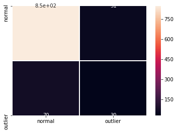
インスタンスレベルの外れ値スコア vs 外れ値閾値をプロットします :
plot_instance_score(od_preds, y_outlier, labels, od.threshold)
isolation forest が外れ値スコアが 0 あたりの外れ値の 1 タイプを検出するのに良い仕事をしていないことが分かります。これは外れ値についての明示的な知識なしに良い閾値を推論することを困難にしています。閾値を 0 のすぐ下に設定することはデータセットの外れ値のために実質的により良い検出性能に繋がるでしょう。これはまた ROC カーブによっても反映されます :
roc_data = {'IF': {'scores': od_preds['data']['instance_score'], 'labels': y_outlier}}
plot_roc(roc_data)
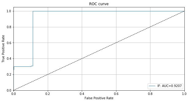
以上
Alibi Detect 0.7 : Examples : マハラノビス外れ値検知 on TCP dump
Alibi Detect 0.7 : Examples : マハラノビス外れ値検知 on KDD Cup ‘99 データセット (翻訳/解説)
翻訳 : (株)クラスキャット セールスインフォメーション
作成日時 : 07/01/2021 (0.7.0)
* 本ページは、Alibi Detect の以下のドキュメントを翻訳した上で適宜、補足説明したものです:
* サンプルコードの動作確認はしておりますが、必要な場合には適宜、追加改変しています。
* ご自由にリンクを張って頂いてかまいませんが、sales-info@classcat.com までご一報いただけると嬉しいです。
スケジュールは弊社 公式 Web サイト でご確認頂けます。
- お住まいの地域に関係なく Web ブラウザからご参加頂けます。事前登録 が必要ですのでご注意ください。
- ウェビナー運用には弊社製品「ClassCat® Webinar」を利用しています。
| 人工知能研究開発支援 | 人工知能研修サービス | テレワーク & オンライン授業を支援 |
| PoC(概念実証)を失敗させないための支援 (本支援はセミナーに参加しアンケートに回答した方を対象としています。) | ||
◆ お問合せ : 本件に関するお問い合わせ先は下記までお願いいたします。
| 株式会社クラスキャット セールス・マーケティング本部 セールス・インフォメーション |
| E-Mail:sales-info@classcat.com ; WebSite: https://www.classcat.com/ ; Facebook |
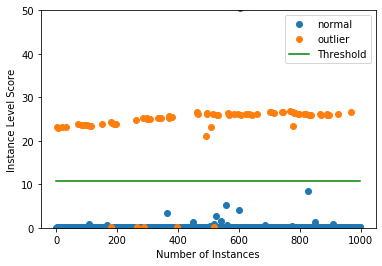
Alibi Detect 0.7 : Examples : マハラノビス外れ値検知 on KDD Cup ‘99 データセット
Mahalanobis 距離 – 概要
マハラノビス・オンライン外れ値検知器は表形式データの異常を予測することが目的です。アルゴリズムは外れ値スコアを計算します、これは特徴分布の中心からの距離の尺度です ( マハラノビス距離 )。外れ値スコアがユーザ定義された閾値より高い場合、観測は外れ値としてフラグ立てされます。このアルゴリズムはオンラインです、これはそれは特徴の分布についての知識なしに開始してリクエストが到着するにつれて学習することを意味しています。結果的に開始時には出力は悪くて時間につれて改良されることを想定するべきです。アルゴリズムは低次元から medium 次元の表形式データに適します。
アルゴリズムはまたカテゴリー (= categorical) 変数を含むこともできます。fit ステップは最初に各カテゴリー変数ののカテゴリー間の pairwise (ペア単位) な距離を計算します。pairwise な距離はモデル予測 (MVDM 法) か (データセットの他の変数により提供される) コンテキスト (ABDM 法) に基づきます。MVDM については、各カテゴリーの条件付きモデル予測確率間の差を使用します。この方法は Cost et al (1993) による Modified Value Difference Metric (MVDM) に基づいています。ABDM は Le et al (2005) により導入されたカテゴリー距離尺度、Association-Based Distance Metric を略しています。ABDM はデータの他の変数の存在からコンテキストを推論して Kullback-Leibler ダイバージェンス に基づいて非類似度 (= dissimilarity measure) を計算します。両者の方法はまた ABDM-MVDM としても結合できます。次に pairwaise 距離をユークリッド空間に射影するために多次元尺度構成法を適用することができます。
データセット
典型的な U.S. 空軍 LAN をシミュレートした LAN の TCP dump データを使用して、外れ値検知器はコンピュータ・ネットワーク侵入を検知する必要があります。コネクションは明確に定義された時間で開始して終了する TCP パケットのシークエンスで、その間にデータは明確に定義されたプロトコルのもとにソース IP とターゲット IP アドレス間で流れます。各コネクションは正常、また攻撃としてラベル付けされます。
データセットには 4 タイプの攻撃があります :
- DOS: denial-of-service, e.g. syn flood;
- R2L: 遠隔マシンからの権限のないアクセス、e.g. パスワードの推測 ;
- U2R: ローカルのスーパーユーザ (root) 特権への権限のないアクセス ;
- probing : 偵察と他の厳密な調査、e.g., ポートスキャン。
データセットは約 500 万のコネクション・レコードを含みます。
3 つのタイプの特徴があります :
- 個々のコネクションの基本的な特徴, e.g. 接続時間 (duration of connection)
- コネクション内のコンテンツ特徴, e.g. 失敗したログイン試行の数
- 2 秒 window 内の traffic 特徴, e.g. 現在の接続と同じホストへのコネクションの数
import matplotlib
%matplotlib inline
import matplotlib.pyplot as plt
import numpy as np
import os
import pandas as pd
import seaborn as sns
from sklearn.metrics import confusion_matrix, f1_score
from sklearn.preprocessing import OneHotEncoder, OrdinalEncoder

from alibi_detect.od import Mahalanobis
from alibi_detect.datasets import fetch_kdd
from alibi_detect.utils.data import create_outlier_batch
from alibi_detect.utils.fetching import fetch_detector
from alibi_detect.utils.mapping import ord2ohe
from alibi_detect.utils.saving import save_detector, load_detector
from alibi_detect.utils.visualize import plot_instance_score, plot_roc
データセットをロードする
幾つかの continuous (連続) な特徴 (41 の内から 18) だけを保持します。
kddcup = fetch_kdd(percent10=True)  # only load 10% of the dataset
print(kddcup.data.shape, kddcup.target.shape)
Downloading https://ndownloader.figshare.com/files/5976042
(494021, 18) (494021,)
kddcup.data[0]
array([8, 0.0, 0.0, 0.0, 0.0, 1.0, 0.0, 0.0, 9, 9, 1.0, 0.0, 0.11, 0.0,
       0.0, 0.0, 0.0, 0.0], dtype=object)
機械学習モデルはデータセットの (外れ値ではなく) 正常インスタンス上で訓練されて標準化 (= standardization) が適用されていると仮定します :
np.random.seed(0)
normal_batch = create_outlier_batch(kddcup.data, kddcup.target, n_samples=100000, perc_outlier=0)
X_train, y_train = normal_batch.data.astype('float'), normal_batch.target
print(X_train.shape, y_train.shape)
print('{}% outliers'.format(100 * y_train.mean()))
(100000, 18) (100000,)
0.0% outliers
mean, stdev = X_train.mean(axis=0), X_train.std(axis=0)
print(mean)
print(stdev)
[1.0863280e+01 1.5947000e-03 1.7106000e-03 5.5465500e-02 5.5817000e-02
 9.8513050e-01 1.8421100e-02 1.3076270e-01 1.4877551e+02 2.0196858e+02
 8.4458450e-01 5.6967800e-02 1.3428810e-01 2.4221900e-02 2.1705000e-03
 1.0195000e-03 5.7662200e-02 5.5782900e-02]
[2.14829720e+01 2.82363937e-02 2.58780186e-02 2.28045718e-01
 2.26992983e-01 9.38338264e-02 1.16618987e-01 2.74664995e-01
 1.03392977e+02 8.70459243e+01 3.06054628e-01 1.81221847e-01
 2.81216847e-01 5.00195618e-02 3.05085878e-02 1.51537329e-02
 2.24991224e-01 2.18815943e-01]
外れ値検知器をロードまたは定義する
examples ノートブックで使用される事前訓練済みの外れ値と敵対的検知器は ここ で見つかります。組込みの fetch_detector 関数を利用できます、これは事前訓練モデルをローカルディレクトリ filepath にセーブして検知器をロードします。代わりに、スクラッチから検知器を初期化できます。
マハラノビスはオンライン、stateful な外れ値検知器であることに注意してください。従ってマハラノビス検知器のセーブやロードはまた検知器の状態もセーブしてロードします。これはユーザに検知器を (それをプロダクションで配備する前に) ウォームアップすることを可能にします。
load_outlier_detector = False
filepath = 'my_path'  # change to directory where model is downloaded
if load_outlier_detector:  # load initialized outlier detector
    detector_type = 'outlier'
    dataset = 'kddcup'
    detector_name = 'Mahalanobis'
    od = fetch_detector(filepath, detector_type, dataset, detector_name)
    filepath = os.path.join(filepath, detector_name)
else:  # initialize and save outlier detector
    threshold = None  # scores above threshold are classified as outliers
    n_components = 2  # nb of components used in PCA
    std_clip = 3  # clip values used to compute mean and cov above "std_clip" standard deviations
    start_clip = 20  # start clipping values after "start_clip" instances

    od = Mahalanobis(threshold,
                     n_components=n_components,
                     std_clip=std_clip,
                     start_clip=start_clip)

    save_detector(od, filepath)  # save outlier detector
No threshold level set. Need to infer threshold using `infer_threshold`.
Directory ./models does not exist and is now created.
!ls model_mahalanobis -l
total 8
-rw-rw-r-- 1 ubuntu ubuntu 182  7月  2 02:39 Mahalanobis.pickle
-rw-rw-r-- 1 ubuntu ubuntu 100  7月  2 02:39 meta.pickle
load_outlier_detector が False に等しい場合、警告が outlier threshold (外れ値閾値) を依然として設定する必要があることを教えてくれます。これは infer_threshold メソッドで成されます。インスタンスのバッチを渡してそれらの何パーセントを正常であると考えるかを threshold_perc を通して指定する必要があります。およそ 5% の外れ値を含むことを知るあるデータを持つと仮定しましょう。外れ値のパーセンテージは create_outlier_batch 関数で perc_outlier で設定できます。
np.random.seed(0)
perc_outlier = 5
threshold_batch = create_outlier_batch(kddcup.data, kddcup.target, n_samples=1000, perc_outlier=perc_outlier)
X_threshold, y_threshold = threshold_batch.data.astype('float'), threshold_batch.target
X_threshold = (X_threshold - mean) / stdev
print('{}% outliers'.format(100 * y_threshold.mean()))
5.0% outliers
od.infer_threshold(X_threshold, threshold_perc=100-perc_outlier)
print('New threshold: {}'.format(od.threshold))
threshold = od.threshold
New threshold: 10.67093404671951
外れ値を検知する
今は 10% の外れ値を持つデータのバッチを生成し、それらを正常データ (inliers) から得られた mean と stdev で標準化し、そしてバッチ内の外れ値を検知します。
np.random.seed(1)
outlier_batch = create_outlier_batch(kddcup.data, kddcup.target, n_samples=1000, perc_outlier=10)
X_outlier, y_outlier = outlier_batch.data.astype('float'), outlier_batch.target
X_outlier = (X_outlier - mean) / stdev
print(X_outlier.shape, y_outlier.shape)
print('{}% outliers'.format(100 * y_outlier.mean()))
(1000, 18) (1000,)
10.0% outliers
外れ値を予測します :
od_preds = od.predict(X_outlier, return_instance_score=True)
type(od_preds)
dict
od_preds.keys()
dict_keys(['data', 'meta'])
od_preds['data'].keys()
dict_keys(['instance_score', 'feature_score', 'is_outlier'])
od_preds['data']['is_outlier'][:10]
array([0, 0, 0, 1, 0, 1, 1, 0, 0, 0])
od_preds['data']['instance_score'][:10]
array([2.03266359e-02, 4.37259911e-02, 1.22390634e-02, 2.31468094e+01,
       1.23040377e-01, 1.66272606e+02, 2.29750258e+01, 6.61924348e-02,
       1.30512869e-01, 1.21724158e-01])
od_preds['data']['feature_score']
(nothing displayed)
今ではウォームアップされた外れ値検知器をセーブできます :
save_detector(od, filepath)
!ls model_mahalanobis -l
total 8
-rw-rw-r-- 1 ubuntu ubuntu 3521  7月  2 02:50 Mahalanobis.pickle
-rw-rw-r-- 1 ubuntu ubuntu  100  7月  2 02:50 meta.pickle
結果を表示する
F1 スコアと混同行列 :
labels = outlier_batch.target_names
y_pred = od_preds['data']['is_outlier']
f1 = f1_score(y_outlier, y_pred)
print('F1 score: {}'.format(f1))
cm = confusion_matrix(y_outlier, y_pred)
df_cm = pd.DataFrame(cm, index=labels, columns=labels)
sns.heatmap(df_cm, annot=True, cbar=True, linewidths=.5)
plt.show()
F1 score: 0.9693877551020408

インスタンスレベルの外れ値スコア vs 外れ値閾値をプロットします :
plot_instance_score(od_preds, y_outlier, labels, od.threshold, ylim=(0,50))
検知器の外れ値スコアのために ROC カーブをプロットできます :
roc_data = {'MD': {'scores': od_preds['data']['instance_score'], 'labels': y_outlier}}
plot_roc(roc_data)
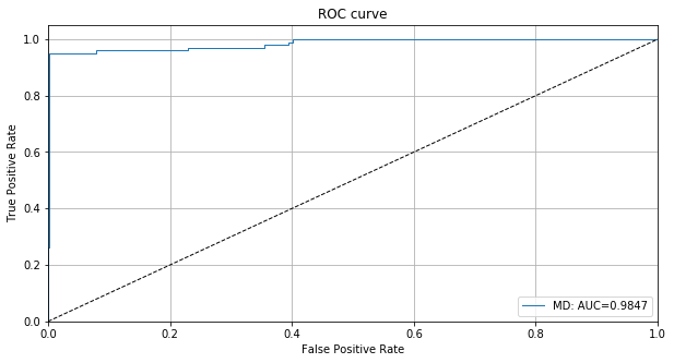
カテゴリー変数を含める
ここまで連続変数だけを追跡しました。けれどもカテゴリー変数を含めることもできます。fit ステップは最初に各カテゴリー変数のカテゴリー間の pairwise 距離を計算します。pairwise 距離はモデル予測 (MVDM メソッド) かデータセットで他の変数により提供されるコンテキスト (ABDM メソッド) に基づいています。MVDM については、各カテゴリーの条件付きモデル予測確率間の差を使用します。この方法は Cost et al (1993) による Modified Value Difference Metric (MVDM) に基づいています。ABDM は Le et al (2005) により導入されたカテゴリー距離尺度、Association-Based Distance Metric を略しています。ABDM はデータの他の変数の存在からコンテキストを推論して Kullback-Leibler ダイバージェンスに基づいて非類似度 (= dissimilarity measure) を計算します。両者の方法はまた ABDM-MVDM としても結合できます。次に pairwaise 距離をユークリッド空間に射影するために多次元尺度構成法を適用することができます。
transform データをロードする
cat_cols = ['protocol_type', 'service', 'flag']
num_cols = ['srv_count', 'serror_rate', 'srv_serror_rate',
            'rerror_rate', 'srv_rerror_rate', 'same_srv_rate',
            'diff_srv_rate', 'srv_diff_host_rate', 'dst_host_count',
            'dst_host_srv_count', 'dst_host_same_srv_rate',
            'dst_host_diff_srv_rate', 'dst_host_same_src_port_rate',
            'dst_host_srv_diff_host_rate', 'dst_host_serror_rate',
            'dst_host_srv_serror_rate', 'dst_host_rerror_rate',
            'dst_host_srv_rerror_rate']
cols = cat_cols + num_cols
np.random.seed(0)
kddcup = fetch_kdd(keep_cols=cols, percent10=True)
print(kddcup.data.shape, kddcup.target.shape)
(494021, 21) (494021,)
キーとしてカテゴリーカラムをそして値としてデータセットの各変数のためのカテゴリー数として辞書を作成します。この辞書は後で外れ値検知器の fit ステップで使用されます。
cat_vars_ord = {}
n_categories = len(cat_cols)
for i in range(n_categories):
    cat_vars_ord[i] = len(np.unique(kddcup.data[:, i]))
print(cat_vars_ord)
{0: 3, 1: 66, 2: 11}
カテゴリーデータ上で ordinal エンコーダを適合します :
enc = OrdinalEncoder()
enc.fit(kddcup.data[:, :n_categories])
OrdinalEncoder(categories='auto', dtype=<class 'numpy.float64'>)
スケールされた数値と ordinal 特徴を組合せます。X_fit はカテゴリー特徴間の距離を推論するために後で使用されます。簡単にするために、後で検知される必要がある外れ値を含め、データセット全体を既に変換しています。これは説明のためです :
X_num = (kddcup.data[:, n_categories:] - mean) / stdev  # standardize numerical features
X_ord = enc.transform(kddcup.data[:, :n_categories])  # apply ordinal encoding to categorical features
X_fit = np.c_[X_ord, X_num].astype(np.float32, copy=False)  # combine numerical and categorical features
print(X_fit.shape)
(494021, 21)
検知器を初期化して適合させる
連続データのためのものと同じ閾値を使用します。これは最適なパフォーマンスという結果にはならないかもしれません。代わりに、閾値を再度推論することもできます。
n_components = 2
std_clip = 3
start_clip = 20

od = Mahalanobis(threshold,
                 n_components=n_components,
                 std_clip=std_clip,
                 start_clip=start_clip,
                 cat_vars=cat_vars_ord,
                 ohe=False)  # True if one-hot encoding (OHE) is used
Set fit parameters:
d_type = 'abdm'  # pairwise distance type, 'abdm' infers context from other variables
disc_perc = [25, 50, 75]  # percentiles used to bin numerical values; used in 'abdm' calculations
standardize_cat_vars = True  # standardize numerical values of categorical variables
カテゴリー変数のために数値を見つけるために fit メソッドを適用します :
od.fit(X_fit,
       d_type=d_type,
       disc_perc=disc_perc,
       standardize_cat_vars=standardize_cat_vars)
カテゴリー特徴のための数値は属性 od.d_abs にストアされます。これはキーとしてカテゴリー特徴のためのカラムをそして値としてカテゴリーの数値と同値のものを持つ辞書です。
cat = 0 # categorical variable to plot numerical values for
plt.bar(np.arange(len(od.d_abs[cat])), od.d_abs[cat])
plt.xticks(np.arange(len(od.d_abs[cat])))
plt.title('Numerical values for categories in categorical variable {}'.format(cat))
plt.xlabel('Category')
plt.ylabel('Numerical value')
plt.show()
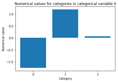
もう一つのオプションはモデルラベル (or 代わりに予測) からカテゴリー変数のための数値を推論するために d_type を ‘mvdm’ にそして y を kddcup.target に設定することです。
外れ値検知器を実行して結果を表示する
10% 外れ値を持つデータのバッチを生成します :
np.random.seed(1)
outlier_batch = create_outlier_batch(kddcup.data, kddcup.target, n_samples=1000, perc_outlier=10)
data, y_outlier = outlier_batch.data, outlier_batch.target
print(data.shape, y_outlier.shape)
print('{}% outliers'.format(100 * y_outlier.mean()))
(1000, 21) (1000,)
10.0% outliers
外れ値バッチを前処理します :
X_num = (data[:, n_categories:] - mean) / stdev
X_ord = enc.transform(data[:, :n_categories])
X_outlier = np.c_[X_ord, X_num].astype(np.float32, copy=False)
print(X_outlier.shape)
(1000, 21)
外れ値を予測します :
od_preds = od.predict(X_outlier, return_instance_score=True)
F1 スコアと混同行列 :
y_pred = od_preds['data']['is_outlier']
f1 = f1_score(y_outlier, y_pred)
print('F1 score: {}'.format(f1))
cm = confusion_matrix(y_outlier, y_pred)
df_cm = pd.DataFrame(cm, index=labels, columns=labels)
sns.heatmap(df_cm, annot=True, cbar=True, linewidths=.5)
plt.show()
F1 score: 0.9375

インスタンス・レベルで外れ値スコア vs 外れ値閾値をプロットします :
plot_instance_score(od_preds, y_outlier, labels, od.threshold, ylim=(0, 150))
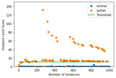
カテゴリー変数のために ordinal エンコーディングの代わりに OHE を使用する
カテゴリー変数上 one-hot エンコーディング (OHE) を適用しますので、cat_vars_ord を ordinal から OHE 形式に変換します。alibi_detect.utils.mapping はこれを行なうためのユティリティ関数を含みます。cat_vars_ohe のキーは今では各 one-hot エンコードされたカテゴリー変数のための最初のカラム・インデックスを表します。この辞書は反事実の説明 (= counterfactual explanation) で後で使用されます。
cat_vars_ohe = ord2ohe(X_fit, cat_vars_ord)[1]
print(cat_vars_ohe)
{0: 3, 3: 66, 69: 11}
カテゴリーデータ上で one-hot エンコーダを適合させます :
enc = OneHotEncoder(categories='auto')
enc.fit(X_fit[:, :n_categories])
OneHotEncoder(categorical_features=None, categories='auto', drop=None,
              dtype=<class 'numpy.float64'>, handle_unknown='error',
              n_values=None, sparse=True)
X_fit を OHE に変換します :
X_ohe = enc.transform(X_fit[:, :n_categories])
X_fit = np.array(np.c_[X_ohe.todense(), X_fit[:, n_categories:]].astype(np.float32, copy=False))
print(X_fit.shape)
(494021, 98)
外れ値検知器を初期化して適合させる
Initialize:
od = Mahalanobis(threshold,
                 n_components=n_components,
                 std_clip=std_clip,
                 start_clip=start_clip,
                 cat_vars=cat_vars_ohe,
                 ohe=True)
fit メソッドを適用します :
od.fit(X_fit,
       d_type=d_type,
       disc_perc=disc_perc,
       standardize_cat_vars=standardize_cat_vars)
外れ値検知器を実行して結果を表示する
外れ値バッチを OHE に変換します :
X_ohe = enc.transform(X_ord)
X_outlier = np.array(np.c_[X_ohe.todense(), X_num].astype(np.float32, copy=False))
print(X_outlier.shape)
(1000, 98)
外れ値を予測します :
od_preds = od.predict(X_outlier, return_instance_score=True)
F1 スコアと混同行列 :
y_pred = od_preds['data']['is_outlier']
f1 = f1_score(y_outlier, y_pred)
print('F1 score: {}'.format(f1))
cm = confusion_matrix(y_outlier, y_pred)
df_cm = pd.DataFrame(cm, index=labels, columns=labels)
sns.heatmap(df_cm, annot=True, cbar=True, linewidths=.5)
plt.show()
F1 score: 0.9375

インスタンスレベルの外れ値スコア vs 外れ値の閾値をプロットします :
plot_instance_score(od_preds, y_outlier, labels, od.threshold, ylim=(0,200))
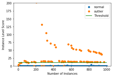
以上
Alibi Detect 0.7 : 概要
Alibi Detect 0.7 : 概要 (翻訳/解説)
翻訳 : (株)クラスキャット セールスインフォメーション
作成日時 : 06/30/2021 (0.7.0)
* 本ページは、Alibi Detect の以下のドキュメントを翻訳した上で適宜、補足説明したものです:
* サンプルコードの動作確認はしておりますが、必要な場合には適宜、追加改変しています。
* ご自由にリンクを張って頂いてかまいませんが、sales-info@classcat.com までご一報いただけると嬉しいです。
スケジュールは弊社 公式 Web サイト でご確認頂けます。
- お住まいの地域に関係なく Web ブラウザからご参加頂けます。事前登録 が必要ですのでご注意ください。
- ウェビナー運用には弊社製品「ClassCat® Webinar」を利用しています。
| 人工知能研究開発支援 | 人工知能研修サービス | テレワーク & オンライン授業を支援 |
| PoC(概念実証)を失敗させないための支援 (本支援はセミナーに参加しアンケートに回答した方を対象としています。) | ||
◆ お問合せ : 本件に関するお問い合わせ先は下記までお願いいたします。
| 株式会社クラスキャット セールス・マーケティング本部 セールス・インフォメーション |
| E-Mail:sales-info@classcat.com ; WebSite: https://www.classcat.com/ ; Facebook |
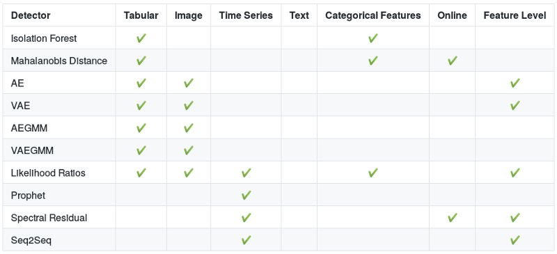
Alibi Detect 0.7 : 概要
Alibi Detect は 外れ値、敵対的 そして ドリフト 検知にフォーカスしたオープンソース Python ライブラリです。このパッケージは表形式データ、テキスト、画像と時系列のためのオンラインとオフライン検知の両者をカバーすることが目的です。TensorFlow と PyTorch バックエンドの両者がドリフト検知のためにサポートされます。
プロダクション設定で外れ値と分布を監視する重要性の背景については、論文 Monitoring and explainability of models in production に基づく、Challenges in Deploying and Monitoring Machine Learning Systems ICML 2020 ワークショップからの このトーク をチェックしてください。
インストールと使用方法
alibi-detect は PyPI からインストールできます :
pip install alibi-detect
代わりに、開発バージョンをインストールすることもできます :
pip install git+https://github.com/SeldonIO/alibi-detect.git
Prophet 時系列外れ値検知器を利用するには :
pip install alibi-detect[prophet]
API を例示するために VAE 外れ値検知を使用します。
from alibi_detect.od import OutlierVAE
from alibi_detect.utils import save_detector, load_detector

# initialize and fit detector
od = OutlierVAE(threshold=0.1, encoder_net=encoder_net, decoder_net=decoder_net, latent_dim=1024)
od.fit(x_train)

# make predictions
preds = od.predict(x_test)

# save and load detectors
filepath = './my_detector/'
save_detector(od, filepath)
od = load_detector(filepath)
予測は meta と data をキーとする辞書で返されます。meta は検出器のメタデータを含む一方で、data は自身の内に実際の予測を持つ辞書です。それは外れ値、敵対的 or ドリフトスコアと閾値、更にはインスタンスが例えば外れ値であるか否かの予測を含みます。正確な詳細はメソッド間で僅かに異なる可能性がありますので、読者には サポートされるアルゴリズムのタイプ に精通することを勧めます。
Prophet 時系列外れ値検知器 のためのセーブとロード機能は現在 Python 3.6 で issue が起きていますが、Python 3.7 では動作します。
サポートされるアルゴリズム
次のテーブルは各アルゴリズムのための推奨ユースケースを示します。カラムの Feature Level (特徴レベル) は検出が特徴レベルで成されるか否かを示します、例えば画像に対してピクセル毎にです。より多くの情報についてはドキュメントと元の論文、そして各々の検出器のためのサンプルへのリンクを持つアルゴリズム参照リストを確認してください。
外れ値検知 (Outlier Detection)
敵対的検出
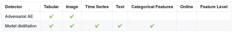
ドリフト検出
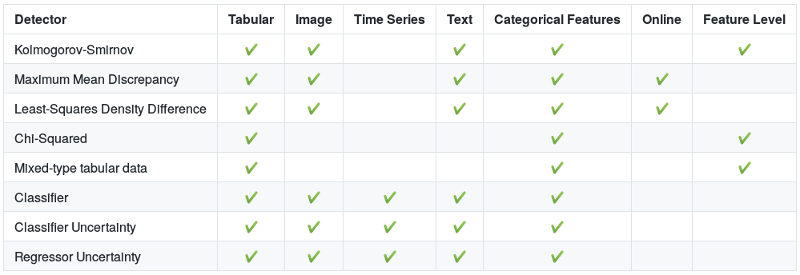
TensorFlow と PyTorch サポート
ドリフト検出器は TensorFlow と PyTorch バックエンドをサポートします。けれども Alibi Detect は PyTorch をインストールしません。これをどのように行なうかは PyTorch docs を確認してください。例えば :
from alibi_detect.cd import MMDDrift
cd = MMDDrift(x_ref, backend='tensorflow', p_val=.05)
preds = cd.predict(x)
PyTorch で同じ検出器 :
cd = MMDDrift(x_ref, backend='pytorch', p_val=.05)
preds = cd.predict(x)
組込みの前処理ステップ
Alibi Detect はまたランダムに初期化されたエンコーダ、transformers ライブラリを使用する際のドリフトを検出するための事前訓練済のテキスト埋め込み、そして機械学習モデルからの隠れ層の抽出のような様々な前処理ステップも装備しています。これは 共変量と予測された分布シフト のような様々なタイプのドリフトを検出することを可能にします。前処理ステップは再び TensorFlow と PyTorch でサポートされます。
from alibi_detect.cd.tensorflow import HiddenOutput, preprocess_drift
model = # TensorFlow model; tf.keras.Model or tf.keras.Sequential
preprocess_fn = partial(preprocess_drift, model=HiddenOutput(model, layer=-1), batch_size=128)
cd = MMDDrift(x_ref, backend='tensorflow', p_val=.05, preprocess_fn=preprocess_fn)
preds = cd.predict(x)
詳細については example ノートブック (e.g. CIFAR10, 映画レビュー) を確認してください。
参照リスト
外れ値検知
- Isolation Forest (FT Liu et al., 2008)
- サンプル: ネットワーク侵入
- マハラノビス距離 (Mahalanobis, 1936)
- サンプル: ネットワーク侵入
- Auto-Encoder (AE)
- サンプル: CIFAR10
- Variational Auto-Encoder (VAE) (Kingma et al., 2013)
- Auto-Encoding ガウス混合モデル (AEGMM) (Zong et al., 2018)
- サンプル: ネットワーク侵入
- 変分 Auto-Encoding ガウス混合モデル (VAEGMM)
- サンプル: ネットワーク侵入
- Likelihood Ratios (尤度比) (Ren et al., 2019)
- サンプル: Genome, Fashion-MNIST vs. MNIST
- Prophet 時系列外れ値検知 (Taylor et al., 2018)
- サンプル: 天気予報
- スペクトル残差 (Spectral Residual) 時系列外れ値検知 (Ren et al., 2019)
- サンプル: 合成データセット
- Sequence-to-Sequence (Seq2Seq) 外れ値検知 (Sutskever et al., 2014; Park et al., 2017)
敵対的検出
- Adversarial Auto-Encoder (Vacanti and Van Looveren, 2020)
- サンプル: CIFAR10
- Model distillation
- サンプル: CIFAR10
ドリフト検出
- Kolmogorov-Smirnov
- Least-Squares Density Difference (Bu et al, 2016)
- Maximum Mean Discrepancy (Gretton et al, 2012)
- Chi-Squared
- サンプル: Income 予測
- Mixed-type 表形式データ
- サンプル: Income 予測
- 分類器 (Lopez-Paz and Oquab, 2017)
- サンプル: CIFAR10
- 分類器と Regressor Uncertainty
- サンプル: CIFAR10 and Wine
- オンライン Maximum Mean Discrepancy
- サンプル: ワイン品質
- オンライン Least-Squares Density Difference (Bu et al, 2017)
- サンプル: ワイン品質
データセット
パッケージはまた様々な多様性のために多くのデータセットを簡単に取得できる alibi_detect.datasets の機能も含みます。各データセットについてデータとラベルか、データ、ラベルとオプションのメタデータを持つ Bunch オブジェクトが返されます。例えば :
from alibi_detect.datasets import fetch_ecg
(X_train, y_train), (X_test, y_test) = fetch_ecg(return_X_y=True)
シーケンシャル・データと時系列
- Genome データセット : fetch_genome
- 分布外分布検出のための尤度率 の一部としてリリースされた、分布外検出のための細菌ゲノム・データセット。オリジナルから TL;DR: データセットは訓練のために 10 in-distribution 細菌クラス、検証のために 60 OOD 細菌クラス、そしてテストのために別の 60 の異なる OOD 細菌クラスからの 250 塩基対のゲノム配列を含みます。訓練、検証とテストセット内にそれぞれ 1, 7 と再び 7 百万のシークエンスがあります。データセットの詳細については、README を確認してください。
from alibi_detect.datasets import fetch_genome (X_train, y_train), (X_val, y_val), (X_test, y_test) = fetch_genome(return_X_y=True)
- 分布外分布検出のための尤度率 の一部としてリリースされた、分布外検出のための細菌ゲノム・データセット。オリジナルから TL;DR: データセットは訓練のために 10 in-distribution 細菌クラス、検証のために 60 OOD 細菌クラス、そしてテストのために別の 60 の異なる OOD 細菌クラスからの 250 塩基対のゲノム配列を含みます。訓練、検証とテストセット内にそれぞれ 1, 7 と再び 7 百万のシークエンスがあります。データセットの詳細については、README を確認してください。
- ECG 5000: fetch_ecg
- Physionet から元は得られた、5000 ECG。
- NAB: fetch_nab
- Numenta 異常値ベンチマーク からの DataFrame 内の単変量時系列。利用可能な時系列を持つリストは alibi_detect.datasets.get_list_nab() を使用して取得できます。使用可能な時系列のリストは、alibi_detect.datasets.get_list_nab()を使用して取得できます。
画像
- CIFAR-10-C: fetch_cifar10c
- CIFAR-10-C (Hendrycks & Dietterich, 2019) は CIFAR-10 のテストセットを含みますが、異なるレベルの重大度 (= severity) で様々なタイプのノイズ、不鮮明さ (=blur)、輝度 etc. により破損 (= corrupted) そして摂動されていて、CIFAR-10 上で訓練された分類モデルのパフォーマンスの段階的な劣化に繋がります。fetch_cifar10c は任意の severity レベルや corruption タイプを選択することを可能にします。利用可能な corruption タイプを持つリストは alibi_detect.datasets.corruption_types_cifar10c() で取得できます。データセットは堅牢性とドリフトの研究で利用できます。元のデータは ここ で見つけられます。例えば :
from alibi_detect.datasets import fetch_cifar10c corruption = ['gaussian_noise', 'motion_blur', 'brightness', 'pixelate'] X, y = fetch_cifar10c(corruption=corruption, severity=5, return_X_y=True)
- CIFAR-10-C (Hendrycks & Dietterich, 2019) は CIFAR-10 のテストセットを含みますが、異なるレベルの重大度 (= severity) で様々なタイプのノイズ、不鮮明さ (=blur)、輝度 etc. により破損 (= corrupted) そして摂動されていて、CIFAR-10 上で訓練された分類モデルのパフォーマンスの段階的な劣化に繋がります。fetch_cifar10c は任意の severity レベルや corruption タイプを選択することを可能にします。利用可能な corruption タイプを持つリストは alibi_detect.datasets.corruption_types_cifar10c() で取得できます。データセットは堅牢性とドリフトの研究で利用できます。元のデータは ここ で見つけられます。例えば :
- 敵対的 CIFAR-10: fetch_attack
- CIFAR-10 で訓練された ResNet-56 分類器上の敵対的インスタンスをロードします。利用可能な攻撃 : Carlini-Wagner (‘cw’) と SLIDE (‘slide’)。例えば :
from alibi_detect.datasets import fetch_attack (X_train, y_train), (X_test, y_test) = fetch_attack('cifar10', 'resnet56', 'cw', return_X_y=True)
- CIFAR-10 で訓練された ResNet-56 分類器上の敵対的インスタンスをロードします。利用可能な攻撃 : Carlini-Wagner (‘cw’) と SLIDE (‘slide’)。例えば :
表形式
- KDD Cup ’99: fetch_kdd
- 様々なタイプのコンピュータ・ネットワーク侵入を伴うデータセット。fetch_kdd はネットワーク侵入のサブセットをターゲットとして選択したり特定の特徴だけを選択することを可能にします。元のデータは ここ で見つけられます。
モデル
外れ値、敵対的あるいはドリフト検出以外で有用であり得るモデル and/or ビルディング・ブロックは alibi_detect.models の下で見つかります。主要な実装は :
- PixelCNN++: alibi_detect.models.pixelcnn.PixelCNN
- 変分 Autoencoder: alibi_detect.models.autoencoder.VAE
- Sequence-to-sequence モデル: alibi_detect.models.autoencoder.Seq2Seq
- ResNet: alibi_detect.models.resnet
- CIFAR-10 上の事前訓練済み ResNet-20/32/44 モデルは Google Cloud Bucket 上で見つけることができて次のように取得できます :
from alibi_detect.utils.fetching import fetch_tf_model model = fetch_tf_model('cifar10', 'resnet32')
- CIFAR-10 上の事前訓練済み ResNet-20/32/44 モデルは Google Cloud Bucket 上で見つけることができて次のように取得できます :
統合
Alibi-detect はオープンソース機械学習モデル配備プラットフォーム Seldon Core とモデルサービング・フレームワーク KFServing に統合されています。
Citations
(訳注 : 原文 を参照してください。)
以上
PyOD 0.8 : Examples : AutoEncoder
PyOD 0.8 : Examples : AutoEncoder (解説)
翻訳 : (株)クラスキャット セールスインフォメーション
作成日時 : 06/28/2021 (0.8.9)
* 本ページは、PyOD の以下のドキュメントとサンプルを参考にして作成しています:
* ご自由にリンクを張って頂いてかまいませんが、sales-info@classcat.com までご一報いただけると嬉しいです。
PyOD 0.8 : Examples : AutoEncoder
完全なサンプル : examples/auto_encoder_example.py
合成データの生成
pyod.utils.data.generate_data() でサンプルデータを生成します :
from pyod.utils.data import generate_data
contamination = 0.1 # percentage of outliers
n_train = 20000 # number of training points
n_test = 2000 # number of testing points
n_features = 300 # number of features
# Generate sample data
X_train, y_train, X_test, y_test = generate_data(
n_train=n_train,
n_test=n_test,
n_features=n_features,
contamination=contamination,
random_state=42)
X_train, y_train の shape と値を確認します :
print(X_train.shape)
print(y_train.shape)
(20000, 300) (20000,)
X_train[:10]
array([[6.43365854, 5.5091683 , 5.04469788, ..., 4.98920813, 6.08796866,
5.65703627],
[6.98114644, 4.97019307, 7.24011768, ..., 4.13407401, 4.17437525,
7.14246591],
[6.96879306, 5.29747338, 5.29666367, ..., 5.97531553, 6.40414268,
5.8399228 ],
...,
[5.13676552, 6.62890142, 6.14075622, ..., 5.42330645, 5.68013833,
7.49193446],
[6.09141558, 5.30143243, 7.09624952, ..., 6.32592813, 7.31717914,
7.4945297 ],
[5.74924769, 6.76427622, 7.10854915, ..., 6.38070765, 6.23367069,
6.3011638 ]])
y_train[:10]
array([0., 0., 0., 0., 0., 0., 0., 0., 0., 0.])
モデル訓練
pyod.models.auto_encoder.AutoEncoder 検出器をインポートして初期化し、そしてモデルを適合させます。
オートエンコーダ (AE) は有用なデータ表現を教師なしで学習するためのニューラルネットワークの一種です。PCA と同様に、再構築エラーを計算することによりデータの外れ値オブジェクトを検出するために使用できるでしょう。
参照 :
- Charu C Aggarwal. Outlier analysis. In Data mining, 75–79. Springer, 2015.
from pyod.models.auto_encoder import AutoEncoder
# train AutoEncoder detector
clf_name = 'AutoEncoder'
clf = AutoEncoder(epochs=30, contamination=contamination)
clf.fit(X_train)
Model: "sequential" _________________________________________________________________ Layer (type) Output Shape Param # ================================================================= dense (Dense) (None, 300) 90300 _________________________________________________________________ dropout (Dropout) (None, 300) 0 _________________________________________________________________ dense_1 (Dense) (None, 300) 90300 _________________________________________________________________ dropout_1 (Dropout) (None, 300) 0 _________________________________________________________________ dense_2 (Dense) (None, 64) 19264 _________________________________________________________________ dropout_2 (Dropout) (None, 64) 0 _________________________________________________________________ dense_3 (Dense) (None, 32) 2080 _________________________________________________________________ dropout_3 (Dropout) (None, 32) 0 _________________________________________________________________ dense_4 (Dense) (None, 32) 1056 _________________________________________________________________ dropout_4 (Dropout) (None, 32) 0 _________________________________________________________________ dense_5 (Dense) (None, 64) 2112 _________________________________________________________________ dropout_5 (Dropout) (None, 64) 0 _________________________________________________________________ dense_6 (Dense) (None, 300) 19500 ================================================================= Total params: 224,612 Trainable params: 224,612 Non-trainable params: 0 _________________________________________________________________ None Epoch 1/30 563/563 [==============================] - 2s 3ms/step - loss: 3.9799 - val_loss: 1.6536 Epoch 2/30 563/563 [==============================] - 1s 2ms/step - loss: 1.3378 - val_loss: 1.2611 Epoch 3/30 563/563 [==============================] - 1s 2ms/step - loss: 1.1653 - val_loss: 1.1830 Epoch 4/30 563/563 [==============================] - 1s 2ms/step - loss: 1.1163 - val_loss: 1.1421 Epoch 5/30 563/563 [==============================] - 1s 2ms/step - loss: 1.0902 - val_loss: 1.1188 Epoch 6/30 563/563 [==============================] - 1s 2ms/step - loss: 1.0745 - val_loss: 1.1108 Epoch 7/30 563/563 [==============================] - 1s 2ms/step - loss: 1.0609 - val_loss: 1.0937 Epoch 8/30 563/563 [==============================] - 1s 2ms/step - loss: 1.0519 - val_loss: 1.0851 Epoch 9/30 563/563 [==============================] - 1s 2ms/step - loss: 1.0439 - val_loss: 1.0823 Epoch 10/30 563/563 [==============================] - 1s 2ms/step - loss: 1.0372 - val_loss: 1.0715 Epoch 11/30 563/563 [==============================] - 1s 2ms/step - loss: 1.0309 - val_loss: 1.0658 Epoch 12/30 563/563 [==============================] - 1s 2ms/step - loss: 1.0247 - val_loss: 1.0612 Epoch 13/30 563/563 [==============================] - 1s 2ms/step - loss: 1.0193 - val_loss: 1.0576 Epoch 14/30 563/563 [==============================] - 1s 2ms/step - loss: 1.0158 - val_loss: 1.0543 Epoch 15/30 563/563 [==============================] - 1s 2ms/step - loss: 1.0129 - val_loss: 1.0523 Epoch 16/30 563/563 [==============================] - 1s 2ms/step - loss: 1.0103 - val_loss: 1.0495 Epoch 17/30 563/563 [==============================] - 1s 2ms/step - loss: 1.0081 - val_loss: 1.0476 Epoch 18/30 563/563 [==============================] - 1s 2ms/step - loss: 1.0062 - val_loss: 1.0460 Epoch 19/30 563/563 [==============================] - 1s 2ms/step - loss: 1.0045 - val_loss: 1.0445 Epoch 20/30 563/563 [==============================] - 1s 2ms/step - loss: 1.0031 - val_loss: 1.0433 Epoch 21/30 563/563 [==============================] - 1s 2ms/step - loss: 1.0019 - val_loss: 1.0422 Epoch 22/30 563/563 [==============================] - 1s 2ms/step - loss: 1.0008 - val_loss: 1.0413 Epoch 23/30 563/563 [==============================] - 1s 2ms/step - loss: 1.0001 - val_loss: 1.0405 Epoch 24/30 563/563 [==============================] - 1s 2ms/step - loss: 0.9993 - val_loss: 1.0399 Epoch 25/30 563/563 [==============================] - 1s 2ms/step - loss: 0.9987 - val_loss: 1.0394 Epoch 26/30 563/563 [==============================] - 1s 2ms/step - loss: 0.9982 - val_loss: 1.0389 Epoch 27/30 563/563 [==============================] - 1s 2ms/step - loss: 0.9978 - val_loss: 1.0386 Epoch 28/30 563/563 [==============================] - 1s 2ms/step - loss: 0.9975 - val_loss: 1.0383 Epoch 29/30 563/563 [==============================] - 1s 2ms/step - loss: 0.9972 - val_loss: 1.0380 Epoch 30/30 563/563 [==============================] - 1s 2ms/step - loss: 0.9969 - val_loss: 1.0378
AutoEncoder(batch_size=32, contamination=0.1, dropout_rate=0.2, epochs=30,
hidden_activation='relu', hidden_neurons=[64, 32, 32, 64],
l2_regularizer=0.1,
loss=,
optimizer='adam', output_activation='sigmoid', preprocessing=True,
random_state=None, validation_size=0.1, verbose=1)
訓練データの予測ラベルと外れ値スコアを取得します :
y_train_pred = clf.labels_ # binary labels (0: inliers, 1: outliers)
y_train_scores = clf.decision_scores_ # raw outlier scores
y_train_pred
array([0, 0, 0, ..., 1, 1, 1])
y_train_scores[:10]
array([7.71661709, 8.3933272 , 8.03062351, 8.3012123 , 7.29930043,
7.8202035 , 8.25040261, 7.89435037, 8.68701496, 7.54829144])
予測と評価
先に正解ラベルを確認しておきます :
y_test
array([0., array([0., 0., 0., ..., 1., 1., 1.])
テストデータ上で予測を行ないます :
y_test_pred = clf.predict(X_test) # outlier labels (0 or 1)
y_test_scores = clf.decision_function(X_test) # outlier scores
y_test_pred
array([0, 0, 0, ..., 1, 1, 1])
y_test_scores[:10]
array([7.88748478, 7.4678574 , 7.68665623, 7.7947202 , 7.81147175,
7.44892412, 7.35455911, 7.74632114, 7.46644309, 8.08000442])
ROC と Precision @ Rank n pyod.utils.data.evaluate_print() を使用して予測を評価します。
from pyod.utils.data import evaluate_print
# evaluate and print the results
print("\nOn Training Data:")
evaluate_print(clf_name, y_train, y_train_scores)
print("\nOn Test Data:")
evaluate_print(clf_name, y_test, y_test_scores)
On Training Data: AutoEncoder ROC:1.0, precision @ rank n:1.0 On Test Data: AutoEncoder ROC:1.0, precision @ rank n:1.0
以上
ClassCat® Chatbot
人工知能開発支援
- テクニカルコンサルティングサービス
- 実証実験 (プロトタイプ構築)
- アプリケーションへの実装
- 人工知能研修サービス
クラスキャット
セールス・インフォメーション
E-Mail:sales-info@classcat.com