ホーム » マハラノビス距離
「マハラノビス距離」カテゴリーアーカイブ
Alibi Detect 0.7 : Examples : マハラノビス外れ値検知 on TCP dump
Alibi Detect 0.7 : Examples : マハラノビス外れ値検知 on KDD Cup ‘99 データセット (翻訳/解説)
翻訳 : (株)クラスキャット セールスインフォメーション
作成日時 : 07/01/2021 (0.7.0)
* 本ページは、Alibi Detect の以下のドキュメントを翻訳した上で適宜、補足説明したものです:
* サンプルコードの動作確認はしておりますが、必要な場合には適宜、追加改変しています。
* ご自由にリンクを張って頂いてかまいませんが、sales-info@classcat.com までご一報いただけると嬉しいです。

スケジュールは弊社 公式 Web サイト でご確認頂けます。
- お住まいの地域に関係なく Web ブラウザからご参加頂けます。事前登録 が必要ですのでご注意ください。
- ウェビナー運用には弊社製品「ClassCat® Webinar」を利用しています。
| 人工知能研究開発支援 | 人工知能研修サービス | テレワーク & オンライン授業を支援 |
| PoC(概念実証)を失敗させないための支援 (本支援はセミナーに参加しアンケートに回答した方を対象としています。) | ||
◆ お問合せ : 本件に関するお問い合わせ先は下記までお願いいたします。
| 株式会社クラスキャット セールス・マーケティング本部 セールス・インフォメーション |
| E-Mail:sales-info@classcat.com ; WebSite: https://www.classcat.com/ ; Facebook |
Alibi Detect 0.7 : Examples : マハラノビス外れ値検知 on KDD Cup ‘99 データセット
Mahalanobis 距離 – 概要
マハラノビス・オンライン外れ値検知器は表形式データの異常を予測することが目的です。アルゴリズムは外れ値スコアを計算します、これは特徴分布の中心からの距離の尺度です ( マハラノビス距離 )。外れ値スコアがユーザ定義された閾値より高い場合、観測は外れ値としてフラグ立てされます。このアルゴリズムはオンラインです、これはそれは特徴の分布についての知識なしに開始してリクエストが到着するにつれて学習することを意味しています。結果的に開始時には出力は悪くて時間につれて改良されることを想定するべきです。アルゴリズムは低次元から medium 次元の表形式データに適します。
アルゴリズムはまたカテゴリー (= categorical) 変数を含むこともできます。fit ステップは最初に各カテゴリー変数ののカテゴリー間の pairwise (ペア単位) な距離を計算します。pairwise な距離はモデル予測 (MVDM 法) か (データセットの他の変数により提供される) コンテキスト (ABDM 法) に基づきます。MVDM については、各カテゴリーの条件付きモデル予測確率間の差を使用します。この方法は Cost et al (1993) による Modified Value Difference Metric (MVDM) に基づいています。ABDM は Le et al (2005) により導入されたカテゴリー距離尺度、Association-Based Distance Metric を略しています。ABDM はデータの他の変数の存在からコンテキストを推論して Kullback-Leibler ダイバージェンス に基づいて非類似度 (= dissimilarity measure) を計算します。両者の方法はまた ABDM-MVDM としても結合できます。次に pairwaise 距離をユークリッド空間に射影するために多次元尺度構成法を適用することができます。
データセット
典型的な U.S. 空軍 LAN をシミュレートした LAN の TCP dump データを使用して、外れ値検知器はコンピュータ・ネットワーク侵入を検知する必要があります。コネクションは明確に定義された時間で開始して終了する TCP パケットのシークエンスで、その間にデータは明確に定義されたプロトコルのもとにソース IP とターゲット IP アドレス間で流れます。各コネクションは正常、また攻撃としてラベル付けされます。
データセットには 4 タイプの攻撃があります :
- DOS: denial-of-service, e.g. syn flood;
- R2L: 遠隔マシンからの権限のないアクセス、e.g. パスワードの推測 ;
- U2R: ローカルのスーパーユーザ (root) 特権への権限のないアクセス ;
- probing : 偵察と他の厳密な調査、e.g., ポートスキャン。
データセットは約 500 万のコネクション・レコードを含みます。
3 つのタイプの特徴があります :
- 個々のコネクションの基本的な特徴, e.g. 接続時間 (duration of connection)
- コネクション内のコンテンツ特徴, e.g. 失敗したログイン試行の数
- 2 秒 window 内の traffic 特徴, e.g. 現在の接続と同じホストへのコネクションの数
import matplotlib
%matplotlib inline
import matplotlib.pyplot as plt
import numpy as np
import os
import pandas as pd
import seaborn as sns
from sklearn.metrics import confusion_matrix, f1_score
from sklearn.preprocessing import OneHotEncoder, OrdinalEncoder

from alibi_detect.od import Mahalanobis
from alibi_detect.datasets import fetch_kdd
from alibi_detect.utils.data import create_outlier_batch
from alibi_detect.utils.fetching import fetch_detector
from alibi_detect.utils.mapping import ord2ohe
from alibi_detect.utils.saving import save_detector, load_detector
from alibi_detect.utils.visualize import plot_instance_score, plot_roc
データセットをロードする
幾つかの continuous (連続) な特徴 (41 の内から 18) だけを保持します。
kddcup = fetch_kdd(percent10=True)  # only load 10% of the dataset
print(kddcup.data.shape, kddcup.target.shape)
Downloading https://ndownloader.figshare.com/files/5976042
(494021, 18) (494021,)
kddcup.data[0]
array([8, 0.0, 0.0, 0.0, 0.0, 1.0, 0.0, 0.0, 9, 9, 1.0, 0.0, 0.11, 0.0,
       0.0, 0.0, 0.0, 0.0], dtype=object)
機械学習モデルはデータセットの (外れ値ではなく) 正常インスタンス上で訓練されて標準化 (= standardization) が適用されていると仮定します :
np.random.seed(0)
normal_batch = create_outlier_batch(kddcup.data, kddcup.target, n_samples=100000, perc_outlier=0)
X_train, y_train = normal_batch.data.astype('float'), normal_batch.target
print(X_train.shape, y_train.shape)
print('{}% outliers'.format(100 * y_train.mean()))
(100000, 18) (100000,)
0.0% outliers
mean, stdev = X_train.mean(axis=0), X_train.std(axis=0)
print(mean)
print(stdev)
[1.0863280e+01 1.5947000e-03 1.7106000e-03 5.5465500e-02 5.5817000e-02
 9.8513050e-01 1.8421100e-02 1.3076270e-01 1.4877551e+02 2.0196858e+02
 8.4458450e-01 5.6967800e-02 1.3428810e-01 2.4221900e-02 2.1705000e-03
 1.0195000e-03 5.7662200e-02 5.5782900e-02]
[2.14829720e+01 2.82363937e-02 2.58780186e-02 2.28045718e-01
 2.26992983e-01 9.38338264e-02 1.16618987e-01 2.74664995e-01
 1.03392977e+02 8.70459243e+01 3.06054628e-01 1.81221847e-01
 2.81216847e-01 5.00195618e-02 3.05085878e-02 1.51537329e-02
 2.24991224e-01 2.18815943e-01]
外れ値検知器をロードまたは定義する
examples ノートブックで使用される事前訓練済みの外れ値と敵対的検知器は ここ で見つかります。組込みの fetch_detector 関数を利用できます、これは事前訓練モデルをローカルディレクトリ filepath にセーブして検知器をロードします。代わりに、スクラッチから検知器を初期化できます。
マハラノビスはオンライン、stateful な外れ値検知器であることに注意してください。従ってマハラノビス検知器のセーブやロードはまた検知器の状態もセーブしてロードします。これはユーザに検知器を (それをプロダクションで配備する前に) ウォームアップすることを可能にします。
load_outlier_detector = False
filepath = 'my_path'  # change to directory where model is downloaded
if load_outlier_detector:  # load initialized outlier detector
    detector_type = 'outlier'
    dataset = 'kddcup'
    detector_name = 'Mahalanobis'
    od = fetch_detector(filepath, detector_type, dataset, detector_name)
    filepath = os.path.join(filepath, detector_name)
else:  # initialize and save outlier detector
    threshold = None  # scores above threshold are classified as outliers
    n_components = 2  # nb of components used in PCA
    std_clip = 3  # clip values used to compute mean and cov above "std_clip" standard deviations
    start_clip = 20  # start clipping values after "start_clip" instances

    od = Mahalanobis(threshold,
                     n_components=n_components,
                     std_clip=std_clip,
                     start_clip=start_clip)

    save_detector(od, filepath)  # save outlier detector
No threshold level set. Need to infer threshold using `infer_threshold`.
Directory ./models does not exist and is now created.
!ls model_mahalanobis -l
total 8
-rw-rw-r-- 1 ubuntu ubuntu 182  7月  2 02:39 Mahalanobis.pickle
-rw-rw-r-- 1 ubuntu ubuntu 100  7月  2 02:39 meta.pickle
load_outlier_detector が False に等しい場合、警告が outlier threshold (外れ値閾値) を依然として設定する必要があることを教えてくれます。これは infer_threshold メソッドで成されます。インスタンスのバッチを渡してそれらの何パーセントを正常であると考えるかを threshold_perc を通して指定する必要があります。およそ 5% の外れ値を含むことを知るあるデータを持つと仮定しましょう。外れ値のパーセンテージは create_outlier_batch 関数で perc_outlier で設定できます。
np.random.seed(0)
perc_outlier = 5
threshold_batch = create_outlier_batch(kddcup.data, kddcup.target, n_samples=1000, perc_outlier=perc_outlier)
X_threshold, y_threshold = threshold_batch.data.astype('float'), threshold_batch.target
X_threshold = (X_threshold - mean) / stdev
print('{}% outliers'.format(100 * y_threshold.mean()))
5.0% outliers
od.infer_threshold(X_threshold, threshold_perc=100-perc_outlier)
print('New threshold: {}'.format(od.threshold))
threshold = od.threshold
New threshold: 10.67093404671951
外れ値を検知する
今は 10% の外れ値を持つデータのバッチを生成し、それらを正常データ (inliers) から得られた mean と stdev で標準化し、そしてバッチ内の外れ値を検知します。
np.random.seed(1)
outlier_batch = create_outlier_batch(kddcup.data, kddcup.target, n_samples=1000, perc_outlier=10)
X_outlier, y_outlier = outlier_batch.data.astype('float'), outlier_batch.target
X_outlier = (X_outlier - mean) / stdev
print(X_outlier.shape, y_outlier.shape)
print('{}% outliers'.format(100 * y_outlier.mean()))
(1000, 18) (1000,)
10.0% outliers
外れ値を予測します :
od_preds = od.predict(X_outlier, return_instance_score=True)
type(od_preds)
dict
od_preds.keys()
dict_keys(['data', 'meta'])
od_preds['data'].keys()
dict_keys(['instance_score', 'feature_score', 'is_outlier'])
od_preds['data']['is_outlier'][:10]
array([0, 0, 0, 1, 0, 1, 1, 0, 0, 0])
od_preds['data']['instance_score'][:10]
array([2.03266359e-02, 4.37259911e-02, 1.22390634e-02, 2.31468094e+01,
       1.23040377e-01, 1.66272606e+02, 2.29750258e+01, 6.61924348e-02,
       1.30512869e-01, 1.21724158e-01])
od_preds['data']['feature_score']
(nothing displayed)
今ではウォームアップされた外れ値検知器をセーブできます :
save_detector(od, filepath)
!ls model_mahalanobis -l
total 8
-rw-rw-r-- 1 ubuntu ubuntu 3521  7月  2 02:50 Mahalanobis.pickle
-rw-rw-r-- 1 ubuntu ubuntu  100  7月  2 02:50 meta.pickle
結果を表示する
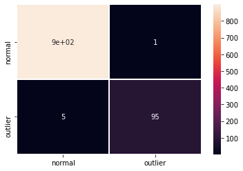
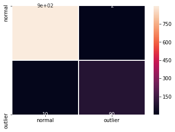
F1 スコアと混同行列 :
labels = outlier_batch.target_names
y_pred = od_preds['data']['is_outlier']
f1 = f1_score(y_outlier, y_pred)
print('F1 score: {}'.format(f1))
cm = confusion_matrix(y_outlier, y_pred)
df_cm = pd.DataFrame(cm, index=labels, columns=labels)
sns.heatmap(df_cm, annot=True, cbar=True, linewidths=.5)
plt.show()
F1 score: 0.9693877551020408
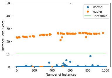
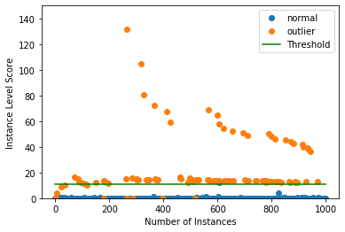
インスタンスレベルの外れ値スコア vs 外れ値閾値をプロットします :
plot_instance_score(od_preds, y_outlier, labels, od.threshold, ylim=(0,50))
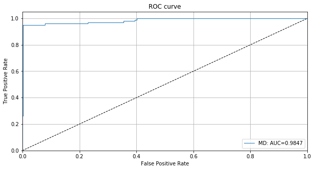
検知器の外れ値スコアのために ROC カーブをプロットできます :
roc_data = {'MD': {'scores': od_preds['data']['instance_score'], 'labels': y_outlier}}
plot_roc(roc_data)
カテゴリー変数を含める
ここまで連続変数だけを追跡しました。けれどもカテゴリー変数を含めることもできます。fit ステップは最初に各カテゴリー変数のカテゴリー間の pairwise 距離を計算します。pairwise 距離はモデル予測 (MVDM メソッド) かデータセットで他の変数により提供されるコンテキスト (ABDM メソッド) に基づいています。MVDM については、各カテゴリーの条件付きモデル予測確率間の差を使用します。この方法は Cost et al (1993) による Modified Value Difference Metric (MVDM) に基づいています。ABDM は Le et al (2005) により導入されたカテゴリー距離尺度、Association-Based Distance Metric を略しています。ABDM はデータの他の変数の存在からコンテキストを推論して Kullback-Leibler ダイバージェンスに基づいて非類似度 (= dissimilarity measure) を計算します。両者の方法はまた ABDM-MVDM としても結合できます。次に pairwaise 距離をユークリッド空間に射影するために多次元尺度構成法を適用することができます。
transform データをロードする
cat_cols = ['protocol_type', 'service', 'flag']
num_cols = ['srv_count', 'serror_rate', 'srv_serror_rate',
            'rerror_rate', 'srv_rerror_rate', 'same_srv_rate',
            'diff_srv_rate', 'srv_diff_host_rate', 'dst_host_count',
            'dst_host_srv_count', 'dst_host_same_srv_rate',
            'dst_host_diff_srv_rate', 'dst_host_same_src_port_rate',
            'dst_host_srv_diff_host_rate', 'dst_host_serror_rate',
            'dst_host_srv_serror_rate', 'dst_host_rerror_rate',
            'dst_host_srv_rerror_rate']
cols = cat_cols + num_cols
np.random.seed(0)
kddcup = fetch_kdd(keep_cols=cols, percent10=True)
print(kddcup.data.shape, kddcup.target.shape)
(494021, 21) (494021,)
キーとしてカテゴリーカラムをそして値としてデータセットの各変数のためのカテゴリー数として辞書を作成します。この辞書は後で外れ値検知器の fit ステップで使用されます。
cat_vars_ord = {}
n_categories = len(cat_cols)
for i in range(n_categories):
    cat_vars_ord[i] = len(np.unique(kddcup.data[:, i]))
print(cat_vars_ord)
{0: 3, 1: 66, 2: 11}
カテゴリーデータ上で ordinal エンコーダを適合します :
enc = OrdinalEncoder()
enc.fit(kddcup.data[:, :n_categories])
OrdinalEncoder(categories='auto', dtype=<class 'numpy.float64'>)
スケールされた数値と ordinal 特徴を組合せます。X_fit はカテゴリー特徴間の距離を推論するために後で使用されます。簡単にするために、後で検知される必要がある外れ値を含め、データセット全体を既に変換しています。これは説明のためです :
X_num = (kddcup.data[:, n_categories:] - mean) / stdev  # standardize numerical features
X_ord = enc.transform(kddcup.data[:, :n_categories])  # apply ordinal encoding to categorical features
X_fit = np.c_[X_ord, X_num].astype(np.float32, copy=False)  # combine numerical and categorical features
print(X_fit.shape)
(494021, 21)
検知器を初期化して適合させる
連続データのためのものと同じ閾値を使用します。これは最適なパフォーマンスという結果にはならないかもしれません。代わりに、閾値を再度推論することもできます。
n_components = 2
std_clip = 3
start_clip = 20

od = Mahalanobis(threshold,
                 n_components=n_components,
                 std_clip=std_clip,
                 start_clip=start_clip,
                 cat_vars=cat_vars_ord,
                 ohe=False)  # True if one-hot encoding (OHE) is used
Set fit parameters:
d_type = 'abdm'  # pairwise distance type, 'abdm' infers context from other variables
disc_perc = [25, 50, 75]  # percentiles used to bin numerical values; used in 'abdm' calculations
standardize_cat_vars = True  # standardize numerical values of categorical variables
カテゴリー変数のために数値を見つけるために fit メソッドを適用します :
od.fit(X_fit,
       d_type=d_type,
       disc_perc=disc_perc,
       standardize_cat_vars=standardize_cat_vars)
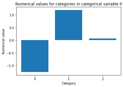
カテゴリー特徴のための数値は属性 od.d_abs にストアされます。これはキーとしてカテゴリー特徴のためのカラムをそして値としてカテゴリーの数値と同値のものを持つ辞書です。
cat = 0 # categorical variable to plot numerical values for
plt.bar(np.arange(len(od.d_abs[cat])), od.d_abs[cat])
plt.xticks(np.arange(len(od.d_abs[cat])))
plt.title('Numerical values for categories in categorical variable {}'.format(cat))
plt.xlabel('Category')
plt.ylabel('Numerical value')
plt.show()
もう一つのオプションはモデルラベル (or 代わりに予測) からカテゴリー変数のための数値を推論するために d_type を ‘mvdm’ にそして y を kddcup.target に設定することです。
外れ値検知器を実行して結果を表示する
10% 外れ値を持つデータのバッチを生成します :
np.random.seed(1)
outlier_batch = create_outlier_batch(kddcup.data, kddcup.target, n_samples=1000, perc_outlier=10)
data, y_outlier = outlier_batch.data, outlier_batch.target
print(data.shape, y_outlier.shape)
print('{}% outliers'.format(100 * y_outlier.mean()))
(1000, 21) (1000,)
10.0% outliers
外れ値バッチを前処理します :
X_num = (data[:, n_categories:] - mean) / stdev
X_ord = enc.transform(data[:, :n_categories])
X_outlier = np.c_[X_ord, X_num].astype(np.float32, copy=False)
print(X_outlier.shape)
(1000, 21)
外れ値を予測します :
od_preds = od.predict(X_outlier, return_instance_score=True)
F1 スコアと混同行列 :
y_pred = od_preds['data']['is_outlier']
f1 = f1_score(y_outlier, y_pred)
print('F1 score: {}'.format(f1))
cm = confusion_matrix(y_outlier, y_pred)
df_cm = pd.DataFrame(cm, index=labels, columns=labels)
sns.heatmap(df_cm, annot=True, cbar=True, linewidths=.5)
plt.show()
F1 score: 0.9375
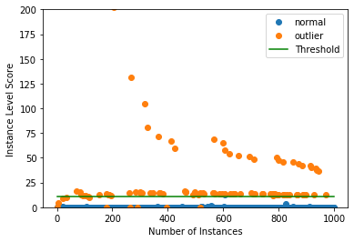
インスタンス・レベルで外れ値スコア vs 外れ値閾値をプロットします :
plot_instance_score(od_preds, y_outlier, labels, od.threshold, ylim=(0, 150))
カテゴリー変数のために ordinal エンコーディングの代わりに OHE を使用する
カテゴリー変数上 one-hot エンコーディング (OHE) を適用しますので、cat_vars_ord を ordinal から OHE 形式に変換します。alibi_detect.utils.mapping はこれを行なうためのユティリティ関数を含みます。cat_vars_ohe のキーは今では各 one-hot エンコードされたカテゴリー変数のための最初のカラム・インデックスを表します。この辞書は反事実の説明 (= counterfactual explanation) で後で使用されます。
cat_vars_ohe = ord2ohe(X_fit, cat_vars_ord)[1]
print(cat_vars_ohe)
{0: 3, 3: 66, 69: 11}
カテゴリーデータ上で one-hot エンコーダを適合させます :
enc = OneHotEncoder(categories='auto')
enc.fit(X_fit[:, :n_categories])
OneHotEncoder(categorical_features=None, categories='auto', drop=None,
              dtype=<class 'numpy.float64'>, handle_unknown='error',
              n_values=None, sparse=True)
X_fit を OHE に変換します :
X_ohe = enc.transform(X_fit[:, :n_categories])
X_fit = np.array(np.c_[X_ohe.todense(), X_fit[:, n_categories:]].astype(np.float32, copy=False))
print(X_fit.shape)
(494021, 98)
外れ値検知器を初期化して適合させる
Initialize:
od = Mahalanobis(threshold,
                 n_components=n_components,
                 std_clip=std_clip,
                 start_clip=start_clip,
                 cat_vars=cat_vars_ohe,
                 ohe=True)
fit メソッドを適用します :
od.fit(X_fit,
       d_type=d_type,
       disc_perc=disc_perc,
       standardize_cat_vars=standardize_cat_vars)
外れ値検知器を実行して結果を表示する
外れ値バッチを OHE に変換します :
X_ohe = enc.transform(X_ord)
X_outlier = np.array(np.c_[X_ohe.todense(), X_num].astype(np.float32, copy=False))
print(X_outlier.shape)
(1000, 98)
外れ値を予測します :
od_preds = od.predict(X_outlier, return_instance_score=True)
F1 スコアと混同行列 :
y_pred = od_preds['data']['is_outlier']
f1 = f1_score(y_outlier, y_pred)
print('F1 score: {}'.format(f1))
cm = confusion_matrix(y_outlier, y_pred)
df_cm = pd.DataFrame(cm, index=labels, columns=labels)
sns.heatmap(df_cm, annot=True, cbar=True, linewidths=.5)
plt.show()
F1 score: 0.9375

インスタンスレベルの外れ値スコア vs 外れ値の閾値をプロットします :
plot_instance_score(od_preds, y_outlier, labels, od.threshold, ylim=(0,200))
以上
PyOD 0.8 : Examples : 最小共分散行列式 (MCD)
PyOD 0.8 : Examples : 最小共分散行列式 (MCD) (解説)
翻訳 : (株)クラスキャット セールスインフォメーション
作成日時 : 06/27/2021 (0.8.9)
* 本ページは、PyOD の以下のドキュメントとサンプルを参考にして作成しています:
* ご自由にリンクを張って頂いてかまいませんが、sales-info@classcat.com までご一報いただけると嬉しいです。
スケジュールは弊社 公式 Web サイト でご確認頂けます。
- お住まいの地域に関係なく Web ブラウザからご参加頂けます。事前登録 が必要ですのでご注意ください。
- ウェビナー運用には弊社製品「ClassCat® Webinar」を利用しています。
| 人工知能研究開発支援 | 人工知能研修サービス | テレワーク & オンライン授業を支援 |
| PoC(概念実証)を失敗させないための支援 (本支援はセミナーに参加しアンケートに回答した方を対象としています。) | ||
◆ お問合せ : 本件に関するお問い合わせ先は下記までお願いいたします。
| 株式会社クラスキャット セールス・マーケティング本部 セールス・インフォメーション |
| E-Mail:sales-info@classcat.com ; WebSite: https://www.classcat.com/ ; Facebook |
PyOD 0.8 : Examples : 最小共分散行列式 (MCD)
完全なサンプル : examples/mcd_example.py
合成データの生成と可視化
pyod.utils.data.generate_data() でサンプルデータを生成します :
from pyod.utils.data import generate_data

contamination = 0.1  # percentage of outliers
n_train = 200  # number of training points
n_test = 100  # number of testing points

X_train, y_train, X_test, y_test = generate_data(
    n_train=n_train, n_test=n_test,
    n_features=2,
    contamination=contamination,
    random_state=42
)
X_train, y_train の shape と値を確認します :
print(X_train.shape)
print(y_train.shape)
(200, 2)
(200,)
X_train[:10]
array([[6.43365854, 5.5091683 ],
       [5.04469788, 7.70806466],
       [5.92453568, 5.25921966],
       [5.29399075, 5.67126197],
       [5.61509076, 6.1309285 ],
       [6.18590347, 6.09410578],
       [7.16630941, 7.22719133],
       [4.05470826, 6.48127032],
       [5.79978164, 5.86930893],
       [4.82256361, 7.18593123]])
y_train[:200]
array([0., 0., 0., 0., 0., 0., 0., 0., 0., 0., 0., 0., 0., 0., 0., 0., 0.,
       0., 0., 0., 0., 0., 0., 0., 0., 0., 0., 0., 0., 0., 0., 0., 0., 0.,
       0., 0., 0., 0., 0., 0., 0., 0., 0., 0., 0., 0., 0., 0., 0., 0., 0.,
       0., 0., 0., 0., 0., 0., 0., 0., 0., 0., 0., 0., 0., 0., 0., 0., 0.,
       0., 0., 0., 0., 0., 0., 0., 0., 0., 0., 0., 0., 0., 0., 0., 0., 0.,
       0., 0., 0., 0., 0., 0., 0., 0., 0., 0., 0., 0., 0., 0., 0., 0., 0.,
       0., 0., 0., 0., 0., 0., 0., 0., 0., 0., 0., 0., 0., 0., 0., 0., 0.,
       0., 0., 0., 0., 0., 0., 0., 0., 0., 0., 0., 0., 0., 0., 0., 0., 0.,
       0., 0., 0., 0., 0., 0., 0., 0., 0., 0., 0., 0., 0., 0., 0., 0., 0.,
       0., 0., 0., 0., 0., 0., 0., 0., 0., 0., 0., 0., 0., 0., 0., 0., 0.,
       0., 0., 0., 0., 0., 0., 0., 0., 0., 0., 1., 1., 1., 1., 1., 1., 1.,
       1., 1., 1., 1., 1., 1., 1., 1., 1., 1., 1., 1., 1.])
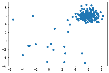
X_train の分布を可視化します :
import matplotlib.pyplot as plt

plt.scatter(X_train[:, 0], X_train[:, 1])
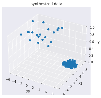
訓練データを可視化します :
import seaborn as sns
sns.set_style("dark")

from mpl_toolkits.mplot3d import Axes3D

X0 = X_train[:, 0]
X1 = X_train[:, 1]
Y = y_train

fig = plt.figure()
ax = Axes3D(fig)

ax.set_title("synthesized data")

ax.set_xlabel("X0")
ax.set_ylabel("X1")
ax.set_zlabel("Y")

ax.plot(X0, X1, Y, marker="o",linestyle='None')
モデル訓練
pyod.models.mcd.MCD 検出器をインポートして初期化し、そしてモデルを適合させます。
最小共分散行列式 (MCD) を使用したガウス分布データセット内の外れ値を検出します : 共分散の堅牢な推定器です。
最小共分散行列式・共分散推定器はガウス分布データ上で適用されますが、単峰性の対称な分布からドローされたデータ上でも関連性がある可能性があります。それは多峰なデータで使用されることを意味していません (MinCovDet オブジェクトを適合させるために使用されるアルゴリズムはそのような場合には失敗する傾向にあります)。多峰なデータセットを処理するためには射影追跡法を考慮するべきです。
最初に最小共分散行列式モデルを適合させてからデータの外れ値の degree として Mahalanobis 距離を計算します。
参照 :
- Johanna Hardin and David M Rocke. Outlier detection in the multiple cluster setting using the minimum covariance determinant estimator. Computational Statistics & Data Analysis, 44(4):625–638, 2004.
- Peter J Rousseeuw and Katrien Van Driessen. A fast algorithm for the minimum covariance determinant estimator. Technometrics, 41(3):212–223, 1999.
from pyod.models.mcd import MCD

clf_name = 'MCD'
clf = MCD()
clf.fit(X_train)
MCD(assume_centered=False, contamination=0.1, random_state=None,
  store_precision=True, support_fraction=None)
訓練データの予測ラベルと外れ値スコアを取得します :
y_train_pred = clf.labels_  # binary labels (0: inliers, 1: outliers)
y_train_scores = clf.decision_scores_  # raw outlier scores
y_train_pred
array([0, 0, 0, 0, 0, 0, 0, 0, 0, 0, 0, 0, 0, 0, 0, 0, 0, 0, 0, 0, 0, 0,
       0, 0, 0, 0, 0, 0, 0, 0, 0, 0, 0, 0, 0, 0, 0, 0, 0, 0, 0, 0, 0, 0,
       0, 0, 0, 0, 0, 0, 0, 0, 0, 0, 1, 0, 0, 0, 0, 0, 0, 0, 0, 0, 0, 0,
       0, 0, 0, 0, 0, 0, 0, 0, 0, 0, 0, 0, 0, 0, 0, 0, 0, 0, 0, 0, 0, 0,
       0, 0, 0, 0, 0, 0, 0, 0, 0, 0, 0, 0, 0, 0, 0, 0, 0, 0, 0, 0, 0, 0,
       0, 0, 0, 0, 0, 0, 0, 0, 0, 0, 0, 0, 0, 0, 0, 0, 0, 0, 0, 0, 0, 0,
       0, 0, 0, 0, 0, 0, 0, 0, 0, 0, 0, 0, 0, 0, 0, 0, 0, 0, 0, 0, 0, 0,
       0, 0, 0, 0, 0, 0, 0, 0, 0, 0, 0, 0, 0, 0, 0, 0, 0, 0, 0, 0, 0, 0,
       0, 0, 0, 0, 1, 1, 1, 1, 1, 1, 1, 1, 1, 1, 0, 1, 1, 1, 1, 1, 1, 1,
       1, 1])
y_train_scores[-40:]
array([4.24565000e+00, 4.22664796e-01, 2.20854837e+00, 3.19271455e+00,
       5.28318116e+00, 4.89035191e+00, 9.00245383e+00, 3.36891011e+00,
       6.41160123e+00, 3.70486129e+00, 8.97553458e-01, 3.23785753e+00,
       3.55922222e-01, 6.19169925e+00, 7.27336532e-01, 3.88522610e+00,
       1.08105367e+00, 1.42204980e+01, 6.55858782e-01, 1.46394676e+00,
       3.95907542e+00, 1.06528255e-01, 6.75944610e-01, 4.94017438e+00,
       5.62629894e+00, 8.14443303e+00, 1.92662344e+00, 7.81555289e+00,
       1.17055228e-01, 6.62232486e-01, 9.36051952e+01, 1.76344612e+02,
       1.03037866e+02, 2.51116697e+02, 1.79382377e+01, 2.37451925e+01,
       1.80881699e+02, 1.72118668e+02, 1.27494937e+02, 6.26970512e+01])
予測と評価
先に正解ラベルを確認しておきます :
y_test
array([0., array([0., 0., 0., 0., 0., 0., 0., 0., 0., 0., 0., 0., 0., 0., 0., 0., 0.,
       0., 0., 0., 0., 0., 0., 0., 0., 0., 0., 0., 0., 0., 0., 0., 0., 0.,
       0., 0., 0., 0., 0., 0., 0., 0., 0., 0., 0., 0., 0., 0., 0., 0., 0.,
       0., 0., 0., 0., 0., 0., 0., 0., 0., 0., 0., 0., 0., 0., 0., 0., 0.,
       0., 0., 0., 0., 0., 0., 0., 0., 0., 0., 0., 0., 0., 0., 0., 0., 0.,
       0., 0., 0., 0., 0., 1., 1., 1., 1., 1., 1., 1., 1., 1., 1.])
テストデータ上で予測を行ないます :
y_test_pred = clf.predict(X_test)  # outlier labels (0 or 1)
y_test_scores = clf.decision_function(X_test)  # outlier scores
y_test_pred
array([0, 0, 0, 0, 0, 0, 0, 0, 0, 0, 0, 0, 0, 0, 0, 0, 0, 0, 0, 0, 0, 0,
       0, 1, 0, 0, 0, 0, 0, 0, 0, 0, 0, 0, 0, 0, 0, 0, 0, 0, 0, 0, 0, 0,
       0, 0, 0, 0, 0, 0, 0, 0, 0, 0, 0, 0, 0, 0, 0, 0, 0, 0, 0, 0, 0, 0,
       0, 0, 0, 0, 0, 0, 0, 0, 0, 0, 0, 1, 0, 0, 0, 0, 0, 0, 0, 0, 0, 0,
       0, 0, 1, 1, 1, 1, 1, 1, 1, 1, 1, 1])
y_test_scores[-40:]
array([ 5.9045124 , -2.01938422, -0.04809363,  1.579808  ,  7.29815783,
        2.75891915, 10.63424239,  1.69629951,  8.35181013,  3.87787154,
       -1.22952342,  2.30787057, -1.92598485,  8.78137251, -1.42671526,
        2.98254633, -1.05400309, 16.91238411, -1.38842923, -1.34779231,
        3.67815253, -1.95072358, -1.54857191,  3.38326885,  8.77706568,
       12.33489833, -0.87534863,  8.73047852, -1.9340466 , -1.4348534 ,
       26.06172492, 25.58479044, 25.93969245, 25.377791  , 22.11729834,
       23.73896701, 25.48826792, 26.29453172, 25.55043239, 25.38483225])
ROC と Precision @ Rank n pyod.utils.data.evaluate_print() を使用して予測を評価します。
from pyod.utils.data import evaluate_print
# evaluate and print the results
print("\nOn Training Data:")
evaluate_print(clf_name, y_train, y_train_scores)
print("\nOn Test Data:")
evaluate_print(clf_name, y_test, y_test_scores)
On Training Data:
MCD ROC:0.9986, precision @ rank n:0.95

On Test Data:
MCD ROC:1.0, precision @ rank n:1.0
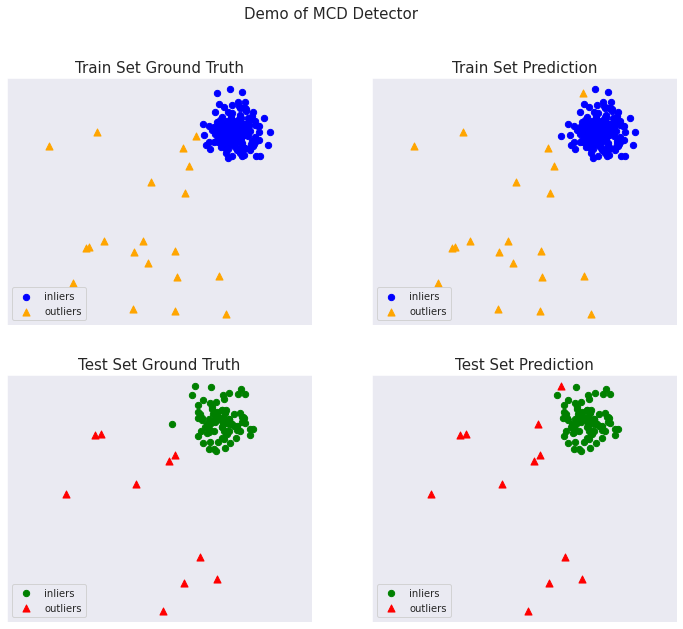
総ての examples に含まれる visualize 関数により可視化を生成します :
from pyod.utils.example import visualize

visualize(clf_name, X_train, y_train, X_test, y_test, y_train_pred,
          y_test_pred, show_figure=True, save_figure=False)
以上
PyOD 0.8 : Examples : k 近傍法 & マハラノビス距離
PyOD 0.8 : Examples : k 近傍法 & マハラノビス距離 (解説)
翻訳 : (株)クラスキャット セールスインフォメーション
作成日時 : 06/26/2021 (0.8.9)
* 本ページは、PyOD の以下のドキュメントとサンプルを参考にして作成しています:
* ご自由にリンクを張って頂いてかまいませんが、sales-info@classcat.com までご一報いただけると嬉しいです。
スケジュールは弊社 公式 Web サイト でご確認頂けます。
- お住まいの地域に関係なく Web ブラウザからご参加頂けます。事前登録 が必要ですのでご注意ください。
- ウェビナー運用には弊社製品「ClassCat® Webinar」を利用しています。
| 人工知能研究開発支援 | 人工知能研修サービス | テレワーク & オンライン授業を支援 |
| PoC(概念実証)を失敗させないための支援 (本支援はセミナーに参加しアンケートに回答した方を対象としています。) | ||
◆ お問合せ : 本件に関するお問い合わせ先は下記までお願いいたします。
| 株式会社クラスキャット セールス・マーケティング本部 セールス・インフォメーション |
| E-Mail:sales-info@classcat.com ; WebSite: https://www.classcat.com/ ; Facebook |
PyOD 0.8 : Examples : k 近傍法 & マハラノビス距離
完全なサンプル : examples/knn_example.py
合成データの生成と可視化
pyod.utils.data.generate_data() でサンプルデータを生成します :
from pyod.utils.data import generate_data

contamination = 0.1  # percentage of outliers
n_train = 200  # number of training points
n_test = 100  # number of testing points

X_train, y_train, X_test, y_test = generate_data(
    n_train=n_train, n_test=n_test, contamination=contamination)
X_train, y_train の shape と値を確認します :
print(X_train.shape)
print(y_train.shape)
(200, 2)
(200,)
X_train[:10]
array([[3.08501648, 4.75998393],
       [4.13746077, 2.48731972],
       [3.79049305, 4.04812774],
       [3.96338469, 4.22143522],
       [4.2801191 , 3.74372575],
       [3.71259428, 3.50012167],
       [5.01925935, 3.85152323],
       [4.30397021, 4.26818773],
       [4.31568536, 3.33965944],
       [3.29025478, 4.32274734]])
y_train[:200]
array([0., 0., 0., 0., 0., 0., 0., 0., 0., 0., 0., 0., 0., 0., 0., 0., 0.,
       0., 0., 0., 0., 0., 0., 0., 0., 0., 0., 0., 0., 0., 0., 0., 0., 0.,
       0., 0., 0., 0., 0., 0., 0., 0., 0., 0., 0., 0., 0., 0., 0., 0., 0.,
       0., 0., 0., 0., 0., 0., 0., 0., 0., 0., 0., 0., 0., 0., 0., 0., 0.,
       0., 0., 0., 0., 0., 0., 0., 0., 0., 0., 0., 0., 0., 0., 0., 0., 0.,
       0., 0., 0., 0., 0., 0., 0., 0., 0., 0., 0., 0., 0., 0., 0., 0., 0.,
       0., 0., 0., 0., 0., 0., 0., 0., 0., 0., 0., 0., 0., 0., 0., 0., 0.,
       0., 0., 0., 0., 0., 0., 0., 0., 0., 0., 0., 0., 0., 0., 0., 0., 0.,
       0., 0., 0., 0., 0., 0., 0., 0., 0., 0., 0., 0., 0., 0., 0., 0., 0.,
       0., 0., 0., 0., 0., 0., 0., 0., 0., 0., 0., 0., 0., 0., 0., 0., 0.,
       0., 0., 0., 0., 0., 0., 0., 0., 0., 0., 1., 1., 1., 1., 1., 1., 1.,
       1., 1., 1., 1., 1., 1., 1., 1., 1., 1., 1., 1., 1.])
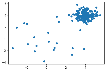
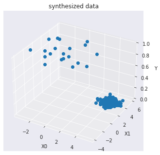
X_train の分布を可視化します :
import matplotlib.pyplot as plt

plt.scatter(X_train[:, 0], X_train[:, 1])
訓練データを可視化します :
import seaborn as sns
sns.set_style("dark")

from mpl_toolkits.mplot3d import Axes3D

X0 = X_train[:, 0]
X1 = X_train[:, 1]
Y = y_train

fig = plt.figure()
ax = Axes3D(fig)

ax.set_title("synthesized data")

ax.set_xlabel("X0")
ax.set_ylabel("X1")
ax.set_zlabel("Y")

ax.plot(X0, X1, Y, marker="o",linestyle='None')
モデル訓練
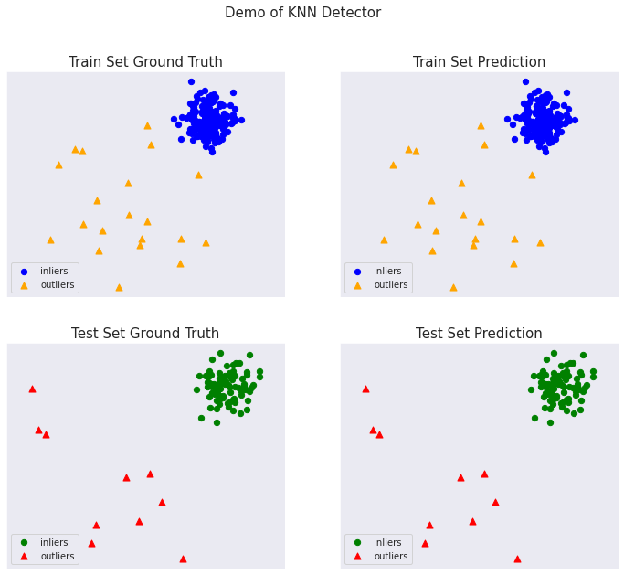
pyod.models.knn.KNN 検出器をインポートして初期化し、そしてモデルを適合させます。
外れ値検知のための kNN クラス。観測について、その k-th 近傍への距離は外れ値スコアとして見なせるでしょう。それは密度を測定する方法としても見なせるでしょう。
参照 :
- Fabrizio Angiulli and Clara Pizzuti. Fast outlier detection in high dimensional spaces. In European Conference on Principles of Data Mining and Knowledge Discovery, 15–27. Springer, 2002.
- Sridhar Ramaswamy, Rajeev Rastogi, and Kyuseok Shim. Efficient algorithms for mining outliers from large data sets. In ACM Sigmod Record, volume 29, 427–438. ACM, 2000.
パラメータ
- method (str, optional (default=’largest’)) – {‘largest’, ‘mean’, ‘median’}
- largest : k-th 近傍への距離を外れ値スコアとして使用します。
- mean : 総ての k 近傍への平均を外れ値スコアとして使用します。
- median : k 近傍への距離の中央値を外れ値スコアとして使用します。
- algorithm ({‘auto’, ‘ball_tree’, ‘kd_tree’, ‘brute’}, optional) –
近傍を計算するために使用されるアルゴリズム :- ’ball_tree’ は BallTree を使用します。
- ’kd_tree’ は KDTree を使用します。
- ’brute’ は brute-force 探索を使用します。
- ’auto’ は fit() メソッドに渡される値を基に最も適切なアルゴリズムを決定することを試みます。
Note: fitting on sparse input will override the setting of this parameter, using brute force.
Deprecated since version 0.74: algorithm is deprecated in PyOD 0.7.4 and will not be possible in 0.7.6. It has to use BallTree for consistency.
- metric (string or callable, default ‘minkowski’) –
距離計算のために使用するメトリック。scikit-learn か scipy.spatial.distance からの任意のメトリックが使用できます。
- metric_params (dict, optional (default = None)) –
metric 関数のための追加のキーワード引数。
from pyod.models.knn import KNN   # kNN detector

# train kNN detector
clf_name = 'KNN'
clf = KNN()
clf.fit(X_train)
KNN(algorithm='auto', contamination=0.1, leaf_size=30, method='largest',
  metric='minkowski', metric_params=None, n_jobs=1, n_neighbors=5, p=2,
  radius=1.0)
訓練データの予測ラベルと外れ値スコアを得ます :
y_train_pred = clf.labels_  # binary labels (0: inliers, 1: outliers)
y_train_scores = clf.decision_scores_  # raw outlier scores
print(y_train_pred)
[0 0 0 0 0 0 0 0 0 0 0 0 0 0 0 0 0 0 0 0 0 0 0 0 0 0 0 0 0 0 0 0 0 0 0 0 0
 0 0 0 0 0 0 0 0 0 0 0 0 0 0 0 0 0 0 0 0 0 0 0 0 0 0 0 0 0 0 0 0 0 0 0 0 0
 0 0 0 0 0 0 0 0 0 0 0 0 0 0 0 0 0 0 0 0 0 0 0 0 0 0 0 0 0 0 0 0 0 0 0 0 0
 0 0 0 0 0 0 0 0 0 0 0 0 0 0 0 0 0 0 0 0 0 0 0 0 0 0 0 0 0 0 0 0 0 0 0 0 0
 0 0 0 0 0 0 0 0 0 0 0 0 0 0 0 0 0 0 0 0 0 0 0 0 0 0 0 0 0 0 0 0 1 1 1 1 1
 1 1 1 1 1 1 1 1 1 1 1 1 1 1 1]
y_train_scores[-40:]
[0.15962472 0.26404758 0.13328626 0.27473931 0.23961003 0.21293019
 0.1147517  0.49774753 0.197176   0.06412986 0.19258264 0.24692469
 0.1676141  0.25805756 0.1975197  0.13500727 0.2091096  0.18331466
 0.25338522 0.23136406 2.38800616 1.9625473  2.10956911 1.8785871
 2.50824404 1.9625473  1.88282016 3.259813   3.05440905 3.36664091
 1.65463831 2.00754852 3.53083084 3.53970455 1.50144057 1.72388028
 2.54678179 3.11133259 2.19112764 1.8785871 ]
予測と評価
正解ラベルを確認しておきます :
y_test
array([0., 0., 0., 0., 0., 0., 0., 0., 0., 0., 0., 0., 0., 0., 0., 0., 0.,
       0., 0., 0., 0., 0., 0., 0., 0., 0., 0., 0., 0., 0., 0., 0., 0., 0.,
       0., 0., 0., 0., 0., 0., 0., 0., 0., 0., 0., 0., 0., 0., 0., 0., 0.,
       0., 0., 0., 0., 0., 0., 0., 0., 0., 0., 0., 0., 0., 0., 0., 0., 0.,
       0., 0., 0., 0., 0., 0., 0., 0., 0., 0., 0., 0., 0., 0., 0., 0., 0.,
       0., 0., 0., 0., 0., 1., 1., 1., 1., 1., 1., 1., 1., 1., 1.])
テストデータ上の予測を行ないます :
y_test_pred = clf.predict(X_test)  # outlier labels (0 or 1)
y_test_scores = clf.decision_function(X_test)  # outlier scores
print(y_test.shape)
y_test_pred
(100,)
[0 0 0 0 0 0 0 0 0 0 0 0 0 0 0 0 0 0 0 0 0 0 0 0 0 0 0 0 0 0 0 0 0 0 0 0 0
 0 0 0 0 0 0 0 0 0 0 0 0 0 0 0 0 0 0 0 0 0 0 0 0 0 0 0 0 0 0 0 0 0 0 0 0 0
 0 0 0 0 0 0 0 0 0 0 0 0 0 0 0 0 1 1 1 1 1 1 1 1 1 1]
y_test_scores[-40:]
array([0.11599486, 0.1838938 , 0.22545484, 0.25303069, 0.19073255,
       0.16952675, 0.27454715, 0.12097446, 0.0909775 , 0.21331808,
       0.13385247, 0.25456906, 0.10869875, 0.13823526, 0.17606727,
       0.19224746, 0.16799589, 0.1532144 , 0.1298472 , 0.30639764,
       0.17532533, 0.22670677, 0.16088692, 0.36243913, 0.17956828,
       0.16300276, 0.08101652, 0.06396358, 0.15957843, 0.62192607,
       3.20652008, 1.97393657, 1.56580327, 1.81336178, 1.54919456,
       2.1308944 , 3.48636464, 2.24250892, 1.87019016, 4.78982494])
ROC と Precision @ Rank n pyod.utils.data.evaluate_print() を使用して予測を評価します。
from pyod.utils.data import evaluate_print
# evaluate and print the results
print("\nOn Training Data:")
evaluate_print(clf_name, y_train, y_train_scores)
print("\nOn Test Data:")
evaluate_print(clf_name, y_test, y_test_scores)
On Training Data:
KNN ROC:1.0, precision @ rank n:1.0

On Test Data:
KNN ROC:1.0, precision @ rank n:1.0
総ての examples に含まれる visualize 関数により可視化を生成します :
from pyod.utils.example import visualize

visualize(clf_name, X_train, y_train, X_test, y_test, y_train_pred,
          y_test_pred, show_figure=True, save_figure=False)
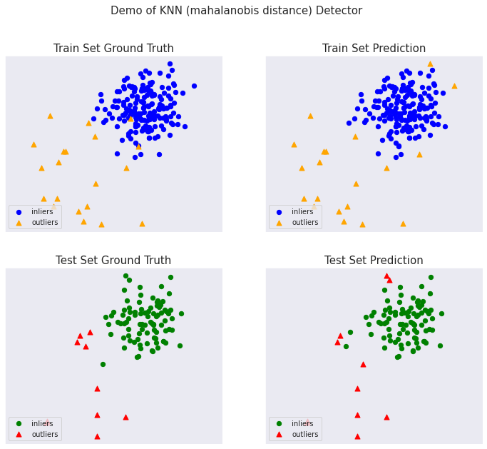
マハラノビス距離
完全なサンプル : examples/knn_mahalanobis_example.py
import numpy as np
from pyod.models.knn import KNN   # kNN detector

# mahalanobis 距離で kNN 検出器を訓練します。
clf_name = 'KNN (mahalanobis distance)'

# calculate covariance for mahalanobis distance
X_train_cov = np.cov(X_train, rowvar=False)
clf = KNN(algorithm='auto', metric='mahalanobis',
              metric_params={'V': X_train_cov})
clf.fit(X_train)
KNN(algorithm='auto', contamination=0.1, leaf_size=30, method='largest',
  metric='mahalanobis',
  metric_params={'V': array([[0.21822, 0.10856],
       [0.10856, 0.223  ]])},
  n_jobs=1, n_neighbors=5, p=2, radius=1.0)
訓練データの予測ラベルと外れ値スコアを得ます :
y_train_pred = clf.labels_  # binary labels (0: inliers, 1: outliers)
y_train_scores = clf.decision_scores_  # raw outlier scores
print(y_train_pred)
[0 0 0 0 0 0 0 0 0 0 0 0 0 1 0 0 0 0 0 0 0 0 0 0 0 0 0 0 0 0 0 0 0 0 0 0 0
 0 0 0 0 0 0 0 0 0 0 0 0 1 0 0 0 0 0 0 0 0 0 0 0 0 0 0 0 0 0 0 0 1 0 0 0 0
 0 0 0 0 0 0 0 0 0 0 0 0 0 0 0 0 0 0 0 0 0 0 0 0 0 0 0 0 0 0 0 0 0 0 0 0 0
 0 0 0 0 0 0 0 0 0 0 0 0 0 0 0 0 0 0 0 0 0 0 0 0 0 0 0 0 0 0 0 0 0 0 0 0 0
 0 0 0 0 0 0 0 0 0 0 0 0 0 0 0 0 0 0 0 0 0 0 0 0 0 0 0 0 0 0 0 0 1 1 1 1 1
 1 1 0 1 1 0 1 1 1 1 1 1 1 0 1]
y_train_scores[-40:]
array([0.58912848, 0.22380705, 0.27005879, 0.41356956, 0.23698991,
       0.26675444, 0.27765579, 0.24205096, 0.15355571, 0.27200349,
       0.26733088, 0.482192  , 0.33874355, 0.25996079, 0.24774249,
       0.1813697 , 0.1223033 , 0.27511716, 0.24852299, 0.20297293,
       1.55753928, 0.80804895, 0.75640102, 1.68413991, 1.63928778,
       1.52363689, 1.4012431 , 0.39888351, 1.36453714, 1.83193458,
       0.66176039, 1.1324612 , 1.33748243, 1.78087079, 1.07614616,
       1.3230474 , 1.37426469, 2.69424388, 0.22668787, 1.22162625])
正解ラベルを確認しておきます :
y_test
array([0., 0., 0., 0., 0., 0., 0., 0., 0., 0., 0., 0., 0., 0., 0., 0., 0.,
       0., 0., 0., 0., 0., 0., 0., 0., 0., 0., 0., 0., 0., 0., 0., 0., 0.,
       0., 0., 0., 0., 0., 0., 0., 0., 0., 0., 0., 0., 0., 0., 0., 0., 0.,
       0., 0., 0., 0., 0., 0., 0., 0., 0., 0., 0., 0., 0., 0., 0., 0., 0.,
       0., 0., 0., 0., 0., 0., 0., 0., 0., 0., 0., 0., 0., 0., 0., 0., 0.,
       0., 0., 0., 0., 0., 1., 1., 1., 1., 1., 1., 1., 1., 1., 1.])
テストデータ上の予測を行ないます :
y_test_pred = clf.predict(X_test)  # outlier labels (0 or 1)
y_test_scores = clf.decision_function(X_test)  # outlier scores
print(y_test.shape)
y_test_pred
(100,)
array([0, 0, 0, 0, 0, 0, 0, 0, 0, 0, 0, 0, 0, 0, 0, 1, 0, 0, 0, 0, 0, 0,
       0, 0, 0, 0, 0, 0, 0, 0, 0, 0, 0, 0, 1, 0, 0, 0, 0, 0, 0, 0, 0, 0,
       0, 0, 0, 0, 0, 0, 0, 0, 0, 0, 0, 0, 0, 0, 0, 0, 0, 0, 0, 0, 0, 0,
       0, 0, 0, 0, 0, 0, 0, 0, 0, 0, 0, 0, 0, 0, 1, 0, 0, 0, 0, 0, 0, 0,
       0, 0, 0, 1, 1, 1, 1, 1, 1, 0, 1, 1])
y_test_scores[-40:]
array([0.21432376, 0.33171001, 0.26295913, 0.18968928, 0.22568313,
       0.43079372, 0.43806264, 0.23698662, 0.56936528, 0.18924124,
       0.20143916, 0.13164876, 0.19035343, 0.28210869, 0.28090227,
       0.32447241, 0.27397147, 0.34668418, 0.29735364, 0.40047555,
       0.7764035 , 0.17145197, 0.38620828, 0.23455709, 0.17468498,
       0.20520947, 0.27625286, 0.18357644, 0.26571843, 0.20382472,
       0.73291695, 1.48326151, 1.04781778, 1.58587852, 1.25507347,
       1.65691819, 0.8926622 , 0.68944944, 1.6565503 , 0.96213366])
ROC と Precision @ Rank n pyod.utils.data.evaluate_print() を使用して予測を評価します。
from pyod.utils.data import evaluate_print
# evaluate and print the results
print("\nOn Training Data:")
evaluate_print(clf_name, y_train, y_train_scores)
print("\nOn Test Data:")
evaluate_print(clf_name, y_test, y_test_scores)
On Training Data:
KNN (mahalanobis distance) ROC:0.9594, precision @ rank n:0.85

On Test Data:
KNN (mahalanobis distance) ROC:0.9889, precision @ rank n:0.8
総ての examples に含まれる visualize 関数により可視化を生成します :
from pyod.utils.example import visualize

visualize(clf_name, X_train, y_train, X_test, y_test, y_train_pred,
          y_test_pred, show_figure=True, save_figure=False)
以上
ClassCat® Chatbot
人工知能開発支援
- テクニカルコンサルティングサービス
- 実証実験 (プロトタイプ構築)
- アプリケーションへの実装
- 人工知能研修サービス
クラスキャット
セールス・インフォメーション
E-Mail:sales-info@classcat.com