Alibi Detect 0.7 : Examples : VAE 外れ値検知 on KDD Cup ‘99 データセット (翻訳/解説)
翻訳 : (株)クラスキャット セールスインフォメーション
作成日時 : 07/02/2021 (0.7.0)
* 本ページは、Alibi Detect の以下のドキュメントを翻訳した上で適宜、補足説明したものです:
* サンプルコードの動作確認はしておりますが、必要な場合には適宜、追加改変しています。
* ご自由にリンクを張って頂いてかまいませんが、sales-info@classcat.com までご一報いただけると嬉しいです。

スケジュールは弊社 公式 Web サイト でご確認頂けます。
- お住まいの地域に関係なく Web ブラウザからご参加頂けます。事前登録 が必要ですのでご注意ください。
- ウェビナー運用には弊社製品「ClassCat® Webinar」を利用しています。
| 人工知能研究開発支援 | 人工知能研修サービス | テレワーク & オンライン授業を支援 |
| PoC(概念実証)を失敗させないための支援 (本支援はセミナーに参加しアンケートに回答した方を対象としています。) | ||
◆ お問合せ : 本件に関するお問い合わせ先は下記までお願いいたします。
| 株式会社クラスキャット セールス・マーケティング本部 セールス・インフォメーション |
| E-Mail:sales-info@classcat.com ; WebSite: https://www.classcat.com/ ; Facebook |
Alibi Detect 0.7 : Examples : VAE 外れ値検知 on KDD Cup ‘99 データセット
VAE – 概要
変分オートエンコーダ (VAE, Variational Auto-Encoder) 外れ値検知器は最初にラベル付けされていない、しかし通常 (inlier) データのバッチで訓練されます。教師なしか半教師あり訓練が望ましいです、何故ならばラベル付けされたデータはしばしば十分でないからです。VAE 検知器はそれが受け取る入力を再構築しようとします。入力データが上手く再構築されない場合、再構築エラーは高くそしてデータは外れ値としてフラグ立てできます。再構築エラーは、入力と再構築されたインスタンスの間の平均二乗誤差 (MSE, mean squared error) か、入力と再構築されたインスタンスの両者が同じプロセスで生成される確率として測定されます。アルゴリズムは表形式か画像データのために適合します。
データセット
典型的な U.S. 空軍 LAN をシミュレートした LAN の TCP dump データを使用して、外れ値検知器はコンピュータ・ネットワーク侵入を検知する必要があります。コネクションは明確に定義された時間で開始して終了する TCP パケットのシークエンスで、その間にデータは明確に定義されたプロトコルのもとにソース IP とターゲット IP アドレス間で流れます。各コネクションは正常、また攻撃としてラベル付けされます。
データセットには 4 タイプの攻撃があります :
- DOS: denial-of-service, e.g. syn flood;
- R2L: 遠隔マシンからの権限のないアクセス、e.g. パスワードの推測 ;
- U2R: ローカルのスーパーユーザ (root) 特権への権限のないアクセス ;
- probing : 偵察と他の厳密な調査、e.g., ポートスキャン。
データセットは約 500 万のコネクション・レコードを含みます。
3 つのタイプの特徴があります :
- 個々のコネクションの基本的な特徴, e.g. 接続時間 (duration of connection)
- コネクション内のコンテンツ特徴, e.g. 失敗したログイン試行の数
- 2 秒 window 内の traffic 特徴, e.g. 現在の接続と同じホストへのコネクションの数
import logging
import matplotlib.pyplot as plt
%matplotlib inline
import numpy as np
import pandas as pd
import seaborn as sns
from sklearn.metrics import confusion_matrix, f1_score
import tensorflow as tf
tf.keras.backend.clear_session()
from tensorflow.keras.layers import Dense, InputLayer

from alibi_detect.datasets import fetch_kdd
from alibi_detect.models.tensorflow.losses import elbo
from alibi_detect.od import OutlierVAE
from alibi_detect.utils.data import create_outlier_batch
from alibi_detect.utils.fetching import fetch_detector
from alibi_detect.utils.saving import save_detector, load_detector
from alibi_detect.utils.visualize import plot_instance_score, plot_feature_outlier_tabular, plot_roc

logger = tf.get_logger()
logger.setLevel(logging.ERROR)
データセットをロードする
幾つかの continuous (連続) な特徴 (41 の内から 18) だけを保持します。
kddcup = fetch_kdd(percent10=True)  # only load 10% of the dataset
print(kddcup.data.shape, kddcup.target.shape)
Downloading https://ndownloader.figshare.com/files/5976042
(494021, 18) (494021,)
kddcup.data[0]
array([8, 0.0, 0.0, 0.0, 0.0, 1.0, 0.0, 0.0, 9, 9, 1.0, 0.0, 0.11, 0.0,
       0.0, 0.0, 0.0, 0.0], dtype=object)
機械学習モデルはデータセットの (外れ値ではなく) 正常インスタンス上で訓練されて標準化 (= standardization) が適用されていると仮定します :
np.random.seed(0)
normal_batch = create_outlier_batch(kddcup.data, kddcup.target, n_samples=400000, perc_outlier=0)
X_train, y_train = normal_batch.data.astype('float'), normal_batch.target
print(X_train.shape, y_train.shape)
print('{}% outliers'.format(100 * y_train.mean()))
(400000, 18) (400000,)
0.0% outliers
mean, stdev = X_train.mean(axis=0), X_train.std(axis=0)
print(mean)
print(stdev)
[1.09550075e+01 1.55620000e-03 1.74745000e-03 5.54626500e-02
 5.57733250e-02 9.85440925e-01 1.82663500e-02 1.33057100e-01
 1.48641492e+02 2.02133175e+02 8.44858050e-01 5.64032750e-02
 1.33479675e-01 2.40508250e-02 2.11637500e-03 1.05915000e-03
 5.73124750e-02 5.52324500e-02]
[2.17181039e+01 2.78305002e-02 2.61481724e-02 2.28073133e-01
 2.26952689e-01 9.25608777e-02 1.16637691e-01 2.77172101e-01
 1.03333220e+02 8.68577798e+01 3.05254458e-01 1.79868747e-01
 2.80221411e-01 4.92476707e-02 2.95181081e-02 1.59275611e-02
 2.24229381e-01 2.17798555e-01]
標準化を適用します :
X_train = (X_train - mean) / stdev
外れ値検知器をロードまたは定義する
examples ノートブックで使用される事前訓練済みの外れ値と敵対的検知器は ここ で見つかります。組込みの fetch_detector 関数を利用できます、これは事前訓練モデルをローカルディレクトリ filepath にセーブして検知器をロードします。代わりに、スクラッチから検知器を訓練することができます。
load_outlier_detector = False
filepath = 'my_dir'  # change to directory (absolute path) where model is downloaded
if load_outlier_detector:  # load pretrained outlier detector
    detector_type = 'outlier'
    dataset = 'kddcup'
    detector_name = 'OutlierVAE'
    od = fetch_detector(filepath, detector_type, dataset, detector_name)
    filepath = os.path.join(filepath, detector_name)
else:  # define model, initialize, train and save outlier detector
    n_features = X_train.shape[1]
    latent_dim = 2

    encoder_net = tf.keras.Sequential(
      [
          InputLayer(input_shape=(n_features,)),
          Dense(20, activation=tf.nn.relu),
          Dense(15, activation=tf.nn.relu),
          Dense(7, activation=tf.nn.relu)
      ])

    decoder_net = tf.keras.Sequential(
      [
          InputLayer(input_shape=(latent_dim,)),
          Dense(7, activation=tf.nn.relu),
          Dense(15, activation=tf.nn.relu),
          Dense(20, activation=tf.nn.relu),
          Dense(n_features, activation=None)
      ])

    # initialize outlier detector
    od = OutlierVAE(threshold=None,  # threshold for outlier score
                    score_type='mse',  # use MSE of reconstruction error for outlier detection
                    encoder_net=encoder_net,  # can also pass VAE model instead
                    decoder_net=decoder_net,  # of separate encoder and decoder
                    latent_dim=latent_dim,
                    samples=5)
    # train
    od.fit(X_train,
           loss_fn=elbo,
           cov_elbo=dict(sim=.01),
           epochs=30,
           verbose=True)

    # save the trained outlier detector
    save_detector(od, filepath)
6250/6250 [=] - 148s 24ms/step - loss: 28695.7242
6250/6250 [=] - 148s 24ms/step - loss: 12437.6854
6250/6250 [=] - 146s 23ms/step - loss: 10256.9219
6250/6250 [=] - 155s 25ms/step - loss: 9557.9839
6250/6250 [=] - 147s 23ms/step - loss: 8414.8731
6250/6250 [=] - 148s 24ms/step - loss: 7847.7130
6250/6250 [=] - 151s 24ms/step - loss: 7549.5546
6250/6250 [=] - 150s 24ms/step - loss: 7412.6179
6250/6250 [=] - 147s 23ms/step - loss: 7358.9181
6250/6250 [=] - 148s 24ms/step - loss: 7064.3351
6250/6250 [=] - 145s 23ms/step - loss: 7047.5733
6250/6250 [=] - 150s 24ms/step - loss: 6862.8724
6250/6250 [=] - 146s 23ms/step - loss: 6859.6950
6250/6250 [=] - 149s 24ms/step - loss: 6733.0950
6250/6250 [=] - 146s 23ms/step - loss: 6395.8519
6250/6250 [=] - 152s 24ms/step - loss: 6239.8235
6250/6250 [=] - 147s 23ms/step - loss: 6141.0218
6250/6250 [=] - 149s 24ms/step - loss: 6080.4994
6250/6250 [=] - 150s 24ms/step - loss: 6030.9626
6250/6250 [=] - 152s 24ms/step - loss: 5986.5710
6250/6250 [=] - 152s 24ms/step - loss: 5968.1871
6250/6250 [=] - 150s 24ms/step - loss: 6026.3471
6250/6250 [=] - 152s 24ms/step - loss: 5828.1424
6250/6250 [=] - 149s 24ms/step - loss: 5841.5844
6250/6250 [=] - 147s 24ms/step - loss: 5794.9508
6250/6250 [=] - 154s 25ms/step - loss: 5792.5575
6250/6250 [=] - 147s 24ms/step - loss: 5767.5592
6250/6250 [=] - 150s 24ms/step - loss: 5643.3078
6250/6250 [=] - 147s 23ms/step - loss: 5571.4557
6250/6250 [=] - 148s 24ms/step - loss: 5541.4037
!ls model_vae -l
!ls model_vae/model -l
total 12
-rw-rw-r-- 1 ubuntu ubuntu  107  7月  2 13:26 OutlierVAE.pickle
-rw-rw-r-- 1 ubuntu ubuntu   87  7月  2 13:26 meta.pickle
drwxrwxr-x 2 ubuntu ubuntu 4096  7月  2 13:26 model
total 64
-rw-rw-r-- 1 ubuntu ubuntu    73  7月  2 13:26 checkpoint
-rw-rw-r-- 1 ubuntu ubuntu 22104  7月  2 13:26 decoder_net.h5
-rw-rw-r-- 1 ubuntu ubuntu 19304  7月  2 13:26 encoder_net.h5
-rw-rw-r-- 1 ubuntu ubuntu  9269  7月  2 13:26 vae.ckpt.data-00000-of-00001
-rw-rw-r-- 1 ubuntu ubuntu  1259  7月  2 13:26 vae.ckpt.index
警告は outlier threshold (外れ値閾値) を依然として設定する必要があることを教えます。これは infer_threshold メソッドで成されます。インスタンスのバッチを渡してそれらの何パーセントを正常であると考えるかを threshold_perc を通して指定する必要があります。およそ 5% の外れ値を含むことを知るあるデータを持つと仮定しましょう。外れ値のパーセンテージは create_outlier_batch 関数で perc_outlier で設定できます。
np.random.seed(0)
perc_outlier = 5
threshold_batch = create_outlier_batch(kddcup.data, kddcup.target, n_samples=1000, perc_outlier=perc_outlier)
X_threshold, y_threshold = threshold_batch.data.astype('float'), threshold_batch.target
X_threshold = (X_threshold - mean) / stdev
print('{}% outliers'.format(100 * y_threshold.mean()))
5.0% outliers
od.infer_threshold(X_threshold, threshold_perc=100-perc_outlier)
print('New threshold: {}'.format(od.threshold))
New threshold: 1.5222603200798008
threshold_perc を例えば 99 に設定して推論された閾値に少しのマージンを加えることにより通常の訓練データから閾値をすいろんすることもできました。更新された閾値で外れ値検知器をセーブしましょう :
save_detector(od, filepath)
!ls model_vae -l
!ls model_vae/model -l
total 12
-rw-rw-r-- 1 ubuntu ubuntu  218  7月  2 13:35 OutlierVAE.pickle
-rw-rw-r-- 1 ubuntu ubuntu   87  7月  2 13:35 meta.pickle
drwxrwxr-x 2 ubuntu ubuntu 4096  7月  2 13:35 model
total 64
-rw-rw-r-- 1 ubuntu ubuntu    73  7月  2 13:35 checkpoint
-rw-rw-r-- 1 ubuntu ubuntu 22104  7月  2 13:35 decoder_net.h5
-rw-rw-r-- 1 ubuntu ubuntu 19304  7月  2 13:35 encoder_net.h5
-rw-rw-r-- 1 ubuntu ubuntu  9269  7月  2 13:35 vae.ckpt.data-00000-of-00001
-rw-rw-r-- 1 ubuntu ubuntu  1259  7月  2 13:35 vae.ckpt.index
外れ値を検出する
今は 10% の外れ値を持つデータのバッチを生成しそしてバッチ内の外れ値を検出します。
np.random.seed(1)
outlier_batch = create_outlier_batch(kddcup.data, kddcup.target, n_samples=1000, perc_outlier=10)
X_outlier, y_outlier = outlier_batch.data.astype('float'), outlier_batch.target
X_outlier = (X_outlier - mean) / stdev
print(X_outlier.shape, y_outlier.shape)
print('{}% outliers'.format(100 * y_outlier.mean()))
(1000, 18) (1000,)
10.0% outliers
外れ値を予測します :
od_preds = od.predict(X_outlier,
                      outlier_type='instance',    # use 'feature' or 'instance' level
                      return_feature_score=True,  # scores used to determine outliers
                      return_instance_score=True)
print(list(od_preds['data'].keys()))
['instance_score', 'feature_score', 'is_outlier']
od_preds['data']['is_outlier'][:10]
array([0, 0, 0, 1, 0, 1, 1, 0, 0, 0])
od_preds['data']['instance_score'][:10]
array([5.74442137e-04, 6.24835379e-04, 6.83877481e-04, 1.52228703e+00,
       2.47923307e-02, 4.29582862e+01, 1.52229905e+00, 4.45219175e-03,
       8.09561496e-02, 2.37765956e-02])
od_preds['data']['feature_score']
array([[4.77347707e-05, 6.23364775e-05, 4.80892692e-05, ...,
        3.21192958e-04, 6.79559419e-05, 5.60611257e-05],
       [1.67435697e-04, 7.68863402e-05, 1.12371712e-04, ...,
        3.19287128e-04, 9.01695907e-05, 8.10840695e-05],
       [9.42410698e-04, 1.08231414e-06, 3.40019366e-05, ...,
        5.65485925e-04, 1.88107799e-05, 1.04572967e-05],
       ...,
       [2.08158688e-03, 4.93670543e-06, 3.57241685e-05, ...,
        6.89739720e-04, 9.91289453e-05, 3.80882650e-06],
       [2.27466705e-03, 4.25181944e-03, 6.06307292e-05, ...,
        3.40673684e-05, 9.27018184e-06, 6.57232246e-03],
       [1.50122506e-03, 4.51257037e-03, 1.09080541e-05, ...,
        4.76422446e-04, 4.67411636e-03, 4.86378648e-02]])
結果を表示する
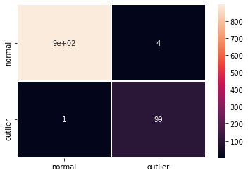
F1 スコアと混同行列 :
labels = outlier_batch.target_names
y_pred = od_preds['data']['is_outlier']
f1 = f1_score(y_outlier, y_pred)
print('F1 score: {:.4f}'.format(f1))
cm = confusion_matrix(y_outlier, y_pred)
df_cm = pd.DataFrame(cm, index=labels, columns=labels)
sns.heatmap(df_cm, annot=True, cbar=True, linewidths=.5)
plt.show()
F1 score: 0.9754
インスタンスレベルの外れ値スコア vs 外れ値閾値をプロットします :
plot_instance_score(od_preds, y_outlier, labels, od.threshold)
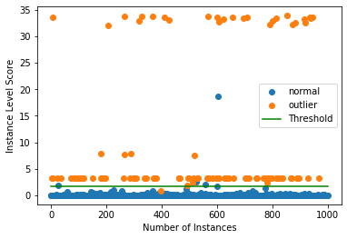
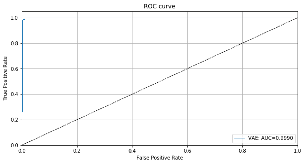
幾つかの外れ値が検出するのに非常に簡単である一方で、他は通常データに近い外れ値スコアを持つことが明瞭に分かります。検出器の外れ値スコアのための ROC カーブをプロットすることもできます :
roc_data = {'VAE': {'scores': od_preds['data']['instance_score'], 'labels': y_outlier}}
plot_roc(roc_data)
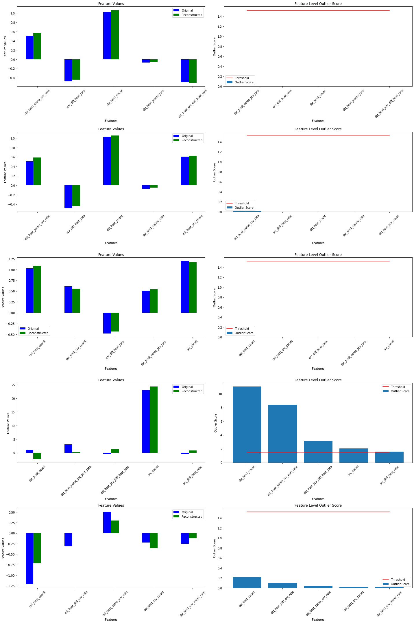
インスタンスレベル外れ値を調査する
今は X_outlier 上の個々の予測の幾つかを詳しく見ることができます。
X_recon = od.vae(X_outlier).numpy() # reconstructed instances by the VAE
plot_feature_outlier_tabular(od_preds,
                             X_outlier,
                             X_recon=X_recon,
                             threshold=od.threshold,
                             instance_ids=None,  # pass a list with indices of instances to display
                             max_instances=5,  # max nb of instances to display
                             top_n=5,  # only show top_n features ordered by outlier score
                             outliers_only=False,  # only show outlier predictions
                             feature_names=kddcup.feature_names,  # add feature names
                             figsize=(20, 30))
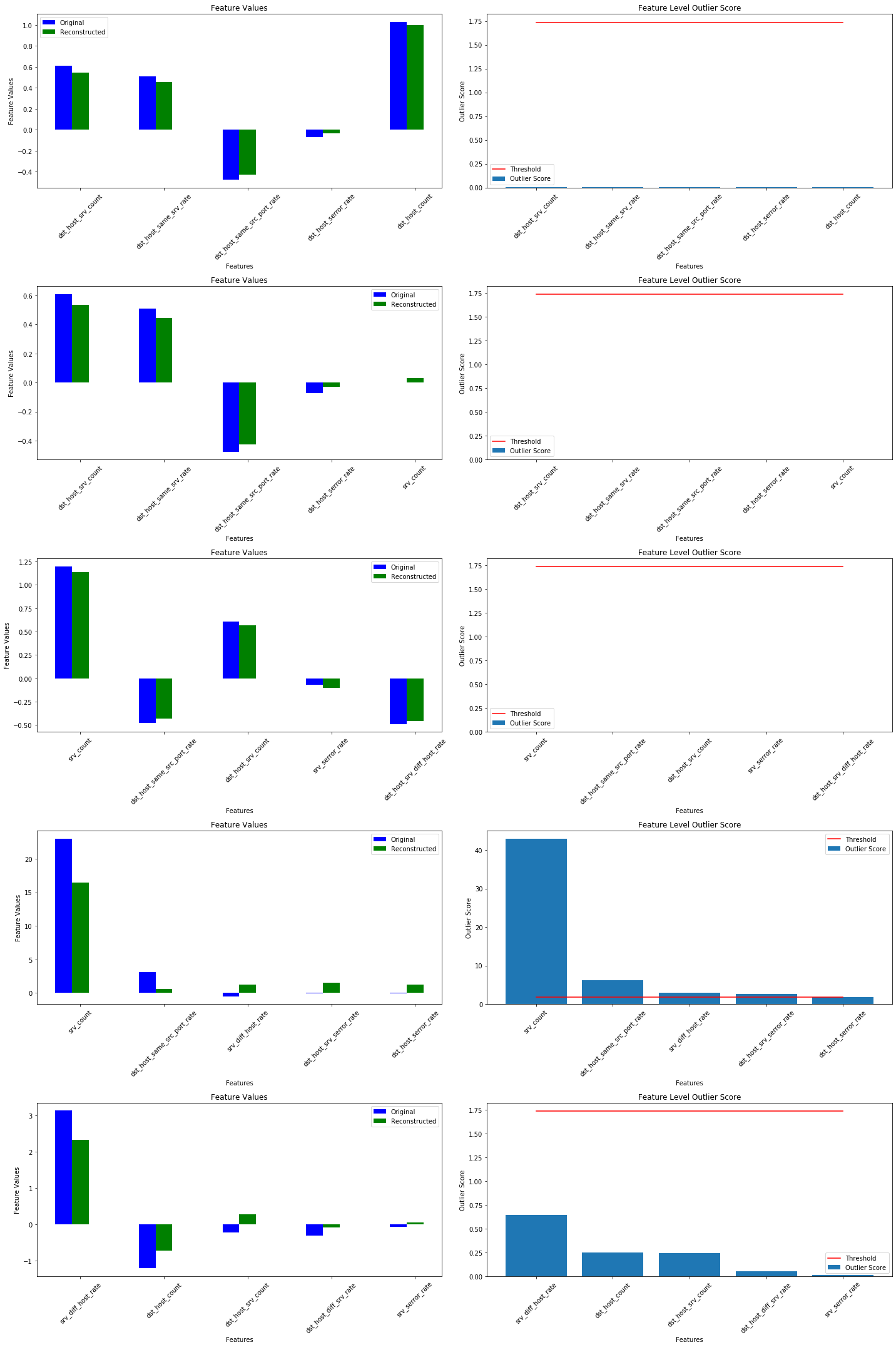
(訳注 : 下は実験結果)
srv_count 特徴は多くの表示される外れ値の責任を負います。
以上