PyOD 0.8 : Examples : 局所外れ値因子 (LOF) (解説)
翻訳 : (株)クラスキャット セールスインフォメーション
作成日時 : 06/28/2021 (0.8.9)
* 本ページは、PyOD の以下のドキュメントとサンプルを参考にして作成しています:
* ご自由にリンクを張って頂いてかまいませんが、sales-info@classcat.com までご一報いただけると嬉しいです。

スケジュールは弊社 公式 Web サイト でご確認頂けます。
- お住まいの地域に関係なく Web ブラウザからご参加頂けます。事前登録 が必要ですのでご注意ください。
- ウェビナー運用には弊社製品「ClassCat® Webinar」を利用しています。
| 人工知能研究開発支援 | 人工知能研修サービス | テレワーク & オンライン授業を支援 |
| PoC(概念実証)を失敗させないための支援 (本支援はセミナーに参加しアンケートに回答した方を対象としています。) | ||
◆ お問合せ : 本件に関するお問い合わせ先は下記までお願いいたします。
| 株式会社クラスキャット セールス・マーケティング本部 セールス・インフォメーション |
| E-Mail:sales-info@classcat.com ; WebSite: https://www.classcat.com/ ; Facebook |
PyOD 0.8 : Examples : 局所外れ値因子 (LOF)
完全なサンプル : examples/lof_example.py
合成データの生成と可視化
pyod.utils.data.generate_data() でサンプルデータを生成します :
from pyod.utils.data import generate_data

contamination = 0.1  # percentage of outliers
n_train = 200  # number of training points
n_test = 100  # number of testing points

X_train, y_train, X_test, y_test = generate_data(
    n_train=n_train, n_test=n_test,
    n_features=2,
    contamination=contamination,
    random_state=42
)
X_train, y_train の shape と値を確認します :
print(X_train.shape)
print(y_train.shape)
(200, 2)
(200,)
X_train[:10]
array([[6.43365854, 5.5091683 ],
       [5.04469788, 7.70806466],
       [5.92453568, 5.25921966],
       [5.29399075, 5.67126197],
       [5.61509076, 6.1309285 ],
       [6.18590347, 6.09410578],
       [7.16630941, 7.22719133],
       [4.05470826, 6.48127032],
       [5.79978164, 5.86930893],
       [4.82256361, 7.18593123]])
y_train[:200]
array([0., 0., 0., 0., 0., 0., 0., 0., 0., 0., 0., 0., 0., 0., 0., 0., 0.,
       0., 0., 0., 0., 0., 0., 0., 0., 0., 0., 0., 0., 0., 0., 0., 0., 0.,
       0., 0., 0., 0., 0., 0., 0., 0., 0., 0., 0., 0., 0., 0., 0., 0., 0.,
       0., 0., 0., 0., 0., 0., 0., 0., 0., 0., 0., 0., 0., 0., 0., 0., 0.,
       0., 0., 0., 0., 0., 0., 0., 0., 0., 0., 0., 0., 0., 0., 0., 0., 0.,
       0., 0., 0., 0., 0., 0., 0., 0., 0., 0., 0., 0., 0., 0., 0., 0., 0.,
       0., 0., 0., 0., 0., 0., 0., 0., 0., 0., 0., 0., 0., 0., 0., 0., 0.,
       0., 0., 0., 0., 0., 0., 0., 0., 0., 0., 0., 0., 0., 0., 0., 0., 0.,
       0., 0., 0., 0., 0., 0., 0., 0., 0., 0., 0., 0., 0., 0., 0., 0., 0.,
       0., 0., 0., 0., 0., 0., 0., 0., 0., 0., 0., 0., 0., 0., 0., 0., 0.,
       0., 0., 0., 0., 0., 0., 0., 0., 0., 0., 1., 1., 1., 1., 1., 1., 1.,
       1., 1., 1., 1., 1., 1., 1., 1., 1., 1., 1., 1., 1.])
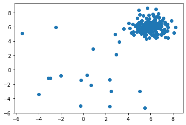
X_train の分布を可視化します :
import matplotlib.pyplot as plt

plt.scatter(X_train[:, 0], X_train[:, 1])
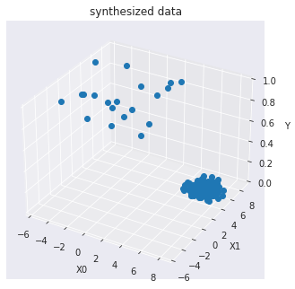
訓練データを可視化します :
import seaborn as sns
sns.set_style("dark")

from mpl_toolkits.mplot3d import Axes3D

X0 = X_train[:, 0]
X1 = X_train[:, 1]
Y = y_train

fig = plt.figure()
ax = Axes3D(fig)

ax.set_title("synthesized data")

ax.set_xlabel("X0")
ax.set_ylabel("X1")
ax.set_zlabel("Y")

ax.plot(X0, X1, Y, marker="o",linestyle='None')
モデル訓練
pyod.models.lof.LOF 検出器をインポートして初期化し、そしてモデルを適合させます。
scikit-learn LOF クラスのより多くの機能を持つラッパーです。局所外れ値因子 (LOF) を使用する教師なし外れ値検知です。
各サンプルの異常スコアは局所外れ値因子と呼ばれます。それは、与えられたサンプルのその近傍に関する密度の局所的な偏差を測定します。 異常スコアが周囲の近傍に関してオブジェクトがどの程度孤立しているかに依存するという点で局所的です。より正確には、局所性は k-近傍により与えられ、その距離は局所密度を推定するために使用されます。サンプルの局所密度をその近傍の局所密度と比較することで、近傍よりも実質的に低い密度を持つサンプルを識別できます。これらは外れ値と考えられます。
参照 :
- Markus M Breunig, Hans-Peter Kriegel, Raymond T Ng, and Jörg Sander. Lof: identifying density-based local outliers. In ACM sigmod record, volume 29, 93–104. ACM, 2000.
from pyod.models.lof import LOF

clf_name = 'LOF'
clf = LOF()
clf.fit(X_train)
LOF(algorithm='auto', contamination=0.1, leaf_size=30, metric='minkowski',
  metric_params=None, n_jobs=1, n_neighbors=20, p=2)
訓練データの予測ラベルと外れ値スコアを取得します :
y_train_pred = clf.labels_  # binary labels (0: inliers, 1: outliers)
y_train_scores = clf.decision_scores_  # raw outlier scores
y_train_pred
array([0, 0, 0, 0, 0, 0, 0, 0, 0, 0, 0, 0, 0, 0, 0, 0, 0, 0, 0, 0, 0, 0,
       0, 0, 0, 0, 0, 0, 0, 0, 0, 0, 0, 0, 0, 0, 0, 0, 0, 0, 0, 0, 0, 0,
       0, 0, 0, 0, 0, 0, 0, 0, 0, 0, 1, 0, 0, 0, 0, 0, 0, 0, 0, 0, 0, 0,
       0, 0, 0, 0, 0, 0, 0, 0, 0, 0, 0, 0, 0, 0, 0, 0, 0, 0, 0, 0, 0, 0,
       0, 0, 0, 0, 0, 0, 0, 0, 0, 0, 0, 0, 0, 0, 0, 0, 0, 0, 0, 0, 0, 0,
       0, 0, 0, 0, 0, 0, 0, 0, 0, 0, 0, 0, 0, 0, 0, 0, 0, 0, 0, 0, 0, 0,
       0, 0, 0, 0, 0, 0, 0, 0, 0, 0, 0, 0, 0, 0, 0, 0, 0, 0, 0, 0, 0, 0,
       0, 0, 0, 0, 0, 0, 0, 0, 0, 0, 0, 0, 0, 0, 0, 0, 0, 0, 0, 0, 0, 0,
       0, 0, 0, 0, 1, 1, 1, 1, 1, 1, 1, 1, 1, 1, 0, 1, 1, 1, 1, 1, 1, 1,
       1, 1])
y_train_scores[-40:]
array([1.0373351 , 1.23270679, 1.09265586, 1.12859822, 1.74295089,
       1.26432797, 1.00387583, 1.32265673, 1.02052867, 1.04926256,
       1.22713433, 1.23132147, 0.95678759, 1.18736669, 1.1196501 ,
       1.22407483, 1.04189977, 0.98252058, 1.01734905, 1.1686789 ,
       2.37922022, 3.21589785, 2.42579873, 2.08097629, 4.79209747,
       3.38198835, 4.6689984 , 2.09441517, 2.88382391, 2.30676828,
       1.91029513, 3.07594268, 4.99950821, 4.45338669, 3.49185524,
       2.30079596, 5.32646346, 3.01951984, 2.92084825, 3.84004143])
予測と評価
先に正解ラベルを確認しておきます :
y_test
array([0., array([0., 0., 0., 0., 0., 0., 0., 0., 0., 0., 0., 0., 0., 0., 0., 0., 0.,
       0., 0., 0., 0., 0., 0., 0., 0., 0., 0., 0., 0., 0., 0., 0., 0., 0.,
       0., 0., 0., 0., 0., 0., 0., 0., 0., 0., 0., 0., 0., 0., 0., 0., 0.,
       0., 0., 0., 0., 0., 0., 0., 0., 0., 0., 0., 0., 0., 0., 0., 0., 0.,
       0., 0., 0., 0., 0., 0., 0., 0., 0., 0., 0., 0., 0., 0., 0., 0., 0.,
       0., 0., 0., 0., 0., 1., 1., 1., 1., 1., 1., 1., 1., 1., 1.])
テストデータ上で予測を行ないます :
y_test_pred = clf.predict(X_test)  # outlier labels (0 or 1)
y_test_scores = clf.decision_function(X_test)  # outlier scores
y_test_pred
array([0, 0, 0, 0, 0, 0, 0, 0, 0, 0, 0, 0, 0, 0, 0, 0, 0, 0, 0, 0, 0, 0,
       0, 1, 0, 0, 0, 0, 0, 0, 0, 0, 0, 0, 0, 0, 0, 0, 0, 0, 0, 0, 0, 0,
       0, 0, 0, 0, 0, 0, 0, 0, 0, 0, 0, 0, 0, 0, 0, 0, 0, 0, 0, 0, 0, 0,
       0, 0, 0, 0, 0, 0, 0, 0, 0, 0, 0, 1, 0, 0, 0, 0, 0, 0, 0, 0, 0, 0,
       0, 0, 1, 1, 1, 1, 1, 1, 1, 1, 1, 1])
y_test_scores[-40:]
array([4.24565000e+00, 4.22664796e-01, 2.20854837e+00, 3.19271455e+00,
       5.28318116e+00, 4.89035191e+00, 9.00245383e+00, 3.36891011e+00,
       6.41160123e+00, 3.70486129e+00, 8.97553458e-01, 3.23785753e+00,
       3.55922222e-01, 6.19169925e+00, 7.27336532e-01, 3.88522610e+00,
       1.08105367e+00, 1.42204980e+01, 6.55858782e-01, 1.46394676e+00,
       3.95907542e+00, 1.06528255e-01, 6.75944610e-01, 4.94017438e+00,
       5.62629894e+00, 8.14443303e+00, 1.92662344e+00, 7.81555289e+00,
       1.17055228e-01, 6.62232486e-01, 9.36051952e+01, 1.76344612e+02,
       1.03037866e+02, 2.51116697e+02, 1.79382377e+01, 2.37451925e+01,
       1.80881699e+02, 1.72118668e+02, 1.27494937e+02, 6.26970512e+01])
ROC と Precision @ Rank n pyod.utils.data.evaluate_print() を使用して予測を評価します。
from pyod.utils.data import evaluate_print
# evaluate and print the results
print("\nOn Training Data:")
evaluate_print(clf_name, y_train, y_train_scores)
print("\nOn Test Data:")
evaluate_print(clf_name, y_test, y_test_scores)
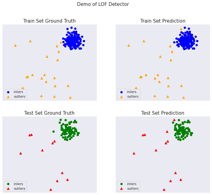
On Training Data:
LOF ROC:0.9997, precision @ rank n:0.95

On Test Data:
LOF ROC:1.0, precision @ rank n:1.0
総ての examples に含まれる visualize 関数により可視化を生成します :
from pyod.utils.example import visualize

visualize(clf_name, X_train, y_train, X_test, y_test, y_train_pred,
          y_test_pred, show_figure=True, save_figure=False)
以上