ホーム » k 近傍法 » PyOD 0.8 : Examples : k 近傍法 & マハラノビス距離

PyOD 0.8 : Examples : k 近傍法 & マハラノビス距離

投稿者: sales-info in k 近傍法, PyOD, マハラノビス距離, 外れ値検知投稿日: 06/26/2021

PyOD 0.8 : Examples : k 近傍法 & マハラノビス距離 (解説)
翻訳 : (株)クラスキャットセールスインフォメーション
作成日時 : 06/26/2021 (0.8.9)

* 本ページは、PyOD の以下のドキュメントとサンプルを参考にして作成しています：

* ご自由にリンクを張って頂いてかまいませんが、sales-info@classcat.com までご一報いただけると嬉しいです。

★ 無料 Web セミナー開催中 ★ クラスキャット主催人工知能 & ビジネス Web セミナー

人工知能とビジネスをテーマに WEB セミナーを定期的に開催しています。
スケジュールは弊社公式 Web サイトでご確認頂けます。

お住まいの地域に関係なく Web ブラウザからご参加頂けます。事前登録 が必要ですのでご注意ください。
ウェビナー運用には弊社製品「ClassCat® Webinar」を利用しています。

クラスキャットは人工知能・テレワークに関する各種サービスを提供しております :

人工知能研究開発支援	人工知能研修サービス	テレワーク & オンライン授業を支援
PoC(概念実証)を失敗させないための支援 (本支援はセミナーに参加しアンケートに回答した方を対象としています。)

◆ お問合せ : 本件に関するお問い合わせ先は下記までお願いいたします。

株式会社クラスキャット セールス・マーケティング本部セールス・インフォメーション

E-Mail：sales-info@classcat.com ; WebSite: https://www.classcat.com/ ; Facebook

PyOD 0.8 : Examples : k 近傍法 & マハラノビス距離

完全なサンプル : examples/knn_example.py

合成データの生成と可視化

pyod.utils.data.generate_data() でサンプルデータを生成します :

from pyod.utils.data import generate_data

contamination = 0.1  # percentage of outliers
n_train = 200  # number of training points
n_test = 100  # number of testing points

X_train, y_train, X_test, y_test = generate_data(
    n_train=n_train, n_test=n_test, contamination=contamination)

X_train, y_train の shape と値を確認します :

print(X_train.shape)
print(y_train.shape)

(200, 2)
(200,)

X_train[:10]

array([[3.08501648, 4.75998393],
       [4.13746077, 2.48731972],
       [3.79049305, 4.04812774],
       [3.96338469, 4.22143522],
       [4.2801191 , 3.74372575],
       [3.71259428, 3.50012167],
       [5.01925935, 3.85152323],
       [4.30397021, 4.26818773],
       [4.31568536, 3.33965944],
       [3.29025478, 4.32274734]])

y_train[:200]

array([0., 0., 0., 0., 0., 0., 0., 0., 0., 0., 0., 0., 0., 0., 0., 0., 0.,
       0., 0., 0., 0., 0., 0., 0., 0., 0., 0., 0., 0., 0., 0., 0., 0., 0.,
       0., 0., 0., 0., 0., 0., 0., 0., 0., 0., 0., 0., 0., 0., 0., 0., 0.,
       0., 0., 0., 0., 0., 0., 0., 0., 0., 0., 0., 0., 0., 0., 0., 0., 0.,
       0., 0., 0., 0., 0., 0., 0., 0., 0., 0., 0., 0., 0., 0., 0., 0., 0.,
       0., 0., 0., 0., 0., 0., 0., 0., 0., 0., 0., 0., 0., 0., 0., 0., 0.,
       0., 0., 0., 0., 0., 0., 0., 0., 0., 0., 0., 0., 0., 0., 0., 0., 0.,
       0., 0., 0., 0., 0., 0., 0., 0., 0., 0., 0., 0., 0., 0., 0., 0., 0.,
       0., 0., 0., 0., 0., 0., 0., 0., 0., 0., 0., 0., 0., 0., 0., 0., 0.,
       0., 0., 0., 0., 0., 0., 0., 0., 0., 0., 0., 0., 0., 0., 0., 0., 0.,
       0., 0., 0., 0., 0., 0., 0., 0., 0., 0., 1., 1., 1., 1., 1., 1., 1.,
       1., 1., 1., 1., 1., 1., 1., 1., 1., 1., 1., 1., 1.])

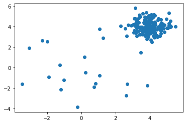
X_train の分布を可視化します :

import matplotlib.pyplot as plt
 
plt.scatter(X_train[:, 0], X_train[:, 1])

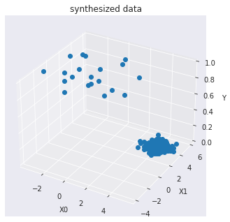
訓練データを可視化します :

import seaborn as sns
sns.set_style("dark")

from mpl_toolkits.mplot3d import Axes3D

X0 = X_train[:, 0]
X1 = X_train[:, 1]
Y = y_train

fig = plt.figure()
ax = Axes3D(fig)

ax.set_title("synthesized data")
 
ax.set_xlabel("X0")
ax.set_ylabel("X1")
ax.set_zlabel("Y")
 
ax.plot(X0, X1, Y, marker="o",linestyle='None')

モデル訓練

pyod.models.knn.KNN 検出器をインポートして初期化し、そしてモデルを適合させます。

外れ値検知のための kNN クラス。観測について、その k-th 近傍への距離は外れ値スコアとして見なせるでしょう。それは密度を測定する方法としても見なせるでしょう。

参照 :

Fabrizio Angiulli and Clara Pizzuti. Fast outlier detection in high dimensional spaces. In European Conference on Principles of Data Mining and Knowledge Discovery, 15–27. Springer, 2002.
Sridhar Ramaswamy, Rajeev Rastogi, and Kyuseok Shim. Efficient algorithms for mining outliers from large data sets. In ACM Sigmod Record, volume 29, 427–438. ACM, 2000.

パラメータ

method (str, optional (default=’largest’)) – {‘largest’, ‘mean’, ‘median’}
- largest : k-th 近傍への距離を外れ値スコアとして使用します。
- mean : 総ての k 近傍への平均を外れ値スコアとして使用します。
- median : k 近傍への距離の中央値を外れ値スコアとして使用します。
algorithm ({‘auto’, ‘ball_tree’, ‘kd_tree’, ‘brute’}, optional) –
近傍を計算するために使用されるアルゴリズム :
- ’ball_tree’ は BallTree を使用します。
- ’kd_tree’ は KDTree を使用します。
- ’brute’ は brute-force 探索を使用します。
- ’auto’ は fit() メソッドに渡される値を基に最も適切なアルゴリズムを決定することを試みます。
Note: fitting on sparse input will override the setting of this parameter, using brute force.

Deprecated since version 0.74: algorithm is deprecated in PyOD 0.7.4 and will not be possible in 0.7.6. It has to use BallTree for consistency.
metric (string or callable, default ‘minkowski’) –
距離計算のために使用するメトリック。scikit-learn か scipy.spatial.distance からの任意のメトリックが使用できます。
metric_params (dict, optional (default = None)) –
metric 関数のための追加のキーワード引数。

from pyod.models.knn import KNN   # kNN detector

# train kNN detector
clf_name = 'KNN'
clf = KNN()
clf.fit(X_train)

KNN(algorithm='auto', contamination=0.1, leaf_size=30, method='largest',
  metric='minkowski', metric_params=None, n_jobs=1, n_neighbors=5, p=2,
  radius=1.0)

訓練データの予測ラベルと外れ値スコアを得ます :

y_train_pred = clf.labels_  # binary labels (0: inliers, 1: outliers)
y_train_scores = clf.decision_scores_  # raw outlier scores

print(y_train_pred)

[0 0 0 0 0 0 0 0 0 0 0 0 0 0 0 0 0 0 0 0 0 0 0 0 0 0 0 0 0 0 0 0 0 0 0 0 0
 0 0 0 0 0 0 0 0 0 0 0 0 0 0 0 0 0 0 0 0 0 0 0 0 0 0 0 0 0 0 0 0 0 0 0 0 0
 0 0 0 0 0 0 0 0 0 0 0 0 0 0 0 0 0 0 0 0 0 0 0 0 0 0 0 0 0 0 0 0 0 0 0 0 0
 0 0 0 0 0 0 0 0 0 0 0 0 0 0 0 0 0 0 0 0 0 0 0 0 0 0 0 0 0 0 0 0 0 0 0 0 0
 0 0 0 0 0 0 0 0 0 0 0 0 0 0 0 0 0 0 0 0 0 0 0 0 0 0 0 0 0 0 0 0 1 1 1 1 1
 1 1 1 1 1 1 1 1 1 1 1 1 1 1 1]

y_train_scores[-40:]

[0.15962472 0.26404758 0.13328626 0.27473931 0.23961003 0.21293019
 0.1147517  0.49774753 0.197176   0.06412986 0.19258264 0.24692469
 0.1676141  0.25805756 0.1975197  0.13500727 0.2091096  0.18331466
 0.25338522 0.23136406 2.38800616 1.9625473  2.10956911 1.8785871
 2.50824404 1.9625473  1.88282016 3.259813   3.05440905 3.36664091
 1.65463831 2.00754852 3.53083084 3.53970455 1.50144057 1.72388028
 2.54678179 3.11133259 2.19112764 1.8785871 ]

予測と評価

正解ラベルを確認しておきます :

y_test

array([0., 0., 0., 0., 0., 0., 0., 0., 0., 0., 0., 0., 0., 0., 0., 0., 0.,
       0., 0., 0., 0., 0., 0., 0., 0., 0., 0., 0., 0., 0., 0., 0., 0., 0.,
       0., 0., 0., 0., 0., 0., 0., 0., 0., 0., 0., 0., 0., 0., 0., 0., 0.,
       0., 0., 0., 0., 0., 0., 0., 0., 0., 0., 0., 0., 0., 0., 0., 0., 0.,
       0., 0., 0., 0., 0., 0., 0., 0., 0., 0., 0., 0., 0., 0., 0., 0., 0.,
       0., 0., 0., 0., 0., 1., 1., 1., 1., 1., 1., 1., 1., 1., 1.])

テストデータ上の予測を行ないます :

y_test_pred = clf.predict(X_test)  # outlier labels (0 or 1)
y_test_scores = clf.decision_function(X_test)  # outlier scores

print(y_test.shape)
y_test_pred

(100,)
[0 0 0 0 0 0 0 0 0 0 0 0 0 0 0 0 0 0 0 0 0 0 0 0 0 0 0 0 0 0 0 0 0 0 0 0 0
 0 0 0 0 0 0 0 0 0 0 0 0 0 0 0 0 0 0 0 0 0 0 0 0 0 0 0 0 0 0 0 0 0 0 0 0 0
 0 0 0 0 0 0 0 0 0 0 0 0 0 0 0 0 1 1 1 1 1 1 1 1 1 1]

y_test_scores[-40:]

array([0.11599486, 0.1838938 , 0.22545484, 0.25303069, 0.19073255,
       0.16952675, 0.27454715, 0.12097446, 0.0909775 , 0.21331808,
       0.13385247, 0.25456906, 0.10869875, 0.13823526, 0.17606727,
       0.19224746, 0.16799589, 0.1532144 , 0.1298472 , 0.30639764,
       0.17532533, 0.22670677, 0.16088692, 0.36243913, 0.17956828,
       0.16300276, 0.08101652, 0.06396358, 0.15957843, 0.62192607,
       3.20652008, 1.97393657, 1.56580327, 1.81336178, 1.54919456,
       2.1308944 , 3.48636464, 2.24250892, 1.87019016, 4.78982494])

ROC と Precision @ Rank n pyod.utils.data.evaluate_print() を使用して予測を評価します。

from pyod.utils.data import evaluate_print
# evaluate and print the results
print("\nOn Training Data:")
evaluate_print(clf_name, y_train, y_train_scores)
print("\nOn Test Data:")
evaluate_print(clf_name, y_test, y_test_scores)

On Training Data:
KNN ROC:1.0, precision @ rank n:1.0

On Test Data:
KNN ROC:1.0, precision @ rank n:1.0

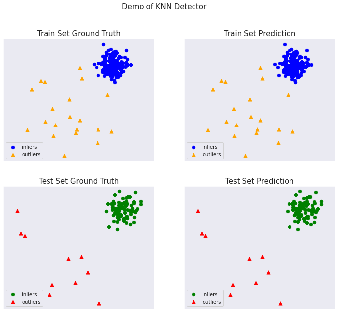
総ての examples に含まれる visualize 関数により可視化を生成します :

from pyod.utils.example import visualize
 
visualize(clf_name, X_train, y_train, X_test, y_test, y_train_pred,
          y_test_pred, show_figure=True, save_figure=False)

マハラノビス距離

完全なサンプル : examples/knn_mahalanobis_example.py

import numpy as np
from pyod.models.knn import KNN   # kNN detector

# mahalanobis 距離で kNN 検出器を訓練します。
clf_name = 'KNN (mahalanobis distance)'

# calculate covariance for mahalanobis distance
X_train_cov = np.cov(X_train, rowvar=False)
clf = KNN(algorithm='auto', metric='mahalanobis',
              metric_params={'V': X_train_cov})
clf.fit(X_train)

KNN(algorithm='auto', contamination=0.1, leaf_size=30, method='largest',
  metric='mahalanobis',
  metric_params={'V': array([[0.21822, 0.10856],
       [0.10856, 0.223  ]])},
  n_jobs=1, n_neighbors=5, p=2, radius=1.0)

訓練データの予測ラベルと外れ値スコアを得ます :

y_train_pred = clf.labels_  # binary labels (0: inliers, 1: outliers)
y_train_scores = clf.decision_scores_  # raw outlier scores

print(y_train_pred)

[0 0 0 0 0 0 0 0 0 0 0 0 0 1 0 0 0 0 0 0 0 0 0 0 0 0 0 0 0 0 0 0 0 0 0 0 0
 0 0 0 0 0 0 0 0 0 0 0 0 1 0 0 0 0 0 0 0 0 0 0 0 0 0 0 0 0 0 0 0 1 0 0 0 0
 0 0 0 0 0 0 0 0 0 0 0 0 0 0 0 0 0 0 0 0 0 0 0 0 0 0 0 0 0 0 0 0 0 0 0 0 0
 0 0 0 0 0 0 0 0 0 0 0 0 0 0 0 0 0 0 0 0 0 0 0 0 0 0 0 0 0 0 0 0 0 0 0 0 0
 0 0 0 0 0 0 0 0 0 0 0 0 0 0 0 0 0 0 0 0 0 0 0 0 0 0 0 0 0 0 0 0 1 1 1 1 1
 1 1 0 1 1 0 1 1 1 1 1 1 1 0 1]

y_train_scores[-40:]

array([0.58912848, 0.22380705, 0.27005879, 0.41356956, 0.23698991,
       0.26675444, 0.27765579, 0.24205096, 0.15355571, 0.27200349,
       0.26733088, 0.482192  , 0.33874355, 0.25996079, 0.24774249,
       0.1813697 , 0.1223033 , 0.27511716, 0.24852299, 0.20297293,
       1.55753928, 0.80804895, 0.75640102, 1.68413991, 1.63928778,
       1.52363689, 1.4012431 , 0.39888351, 1.36453714, 1.83193458,
       0.66176039, 1.1324612 , 1.33748243, 1.78087079, 1.07614616,
       1.3230474 , 1.37426469, 2.69424388, 0.22668787, 1.22162625])

正解ラベルを確認しておきます :

y_test

array([0., 0., 0., 0., 0., 0., 0., 0., 0., 0., 0., 0., 0., 0., 0., 0., 0.,
       0., 0., 0., 0., 0., 0., 0., 0., 0., 0., 0., 0., 0., 0., 0., 0., 0.,
       0., 0., 0., 0., 0., 0., 0., 0., 0., 0., 0., 0., 0., 0., 0., 0., 0.,
       0., 0., 0., 0., 0., 0., 0., 0., 0., 0., 0., 0., 0., 0., 0., 0., 0.,
       0., 0., 0., 0., 0., 0., 0., 0., 0., 0., 0., 0., 0., 0., 0., 0., 0.,
       0., 0., 0., 0., 0., 1., 1., 1., 1., 1., 1., 1., 1., 1., 1.])

テストデータ上の予測を行ないます :

y_test_pred = clf.predict(X_test)  # outlier labels (0 or 1)
y_test_scores = clf.decision_function(X_test)  # outlier scores

print(y_test.shape)
y_test_pred

(100,)
array([0, 0, 0, 0, 0, 0, 0, 0, 0, 0, 0, 0, 0, 0, 0, 1, 0, 0, 0, 0, 0, 0,
       0, 0, 0, 0, 0, 0, 0, 0, 0, 0, 0, 0, 1, 0, 0, 0, 0, 0, 0, 0, 0, 0,
       0, 0, 0, 0, 0, 0, 0, 0, 0, 0, 0, 0, 0, 0, 0, 0, 0, 0, 0, 0, 0, 0,
       0, 0, 0, 0, 0, 0, 0, 0, 0, 0, 0, 0, 0, 0, 1, 0, 0, 0, 0, 0, 0, 0,
       0, 0, 0, 1, 1, 1, 1, 1, 1, 0, 1, 1])

y_test_scores[-40:]

array([0.21432376, 0.33171001, 0.26295913, 0.18968928, 0.22568313,
       0.43079372, 0.43806264, 0.23698662, 0.56936528, 0.18924124,
       0.20143916, 0.13164876, 0.19035343, 0.28210869, 0.28090227,
       0.32447241, 0.27397147, 0.34668418, 0.29735364, 0.40047555,
       0.7764035 , 0.17145197, 0.38620828, 0.23455709, 0.17468498,
       0.20520947, 0.27625286, 0.18357644, 0.26571843, 0.20382472,
       0.73291695, 1.48326151, 1.04781778, 1.58587852, 1.25507347,
       1.65691819, 0.8926622 , 0.68944944, 1.6565503 , 0.96213366])

ROC と Precision @ Rank n pyod.utils.data.evaluate_print() を使用して予測を評価します。

from pyod.utils.data import evaluate_print
# evaluate and print the results
print("\nOn Training Data:")
evaluate_print(clf_name, y_train, y_train_scores)
print("\nOn Test Data:")
evaluate_print(clf_name, y_test, y_test_scores)

On Training Data:
KNN (mahalanobis distance) ROC:0.9594, precision @ rank n:0.85

On Test Data:
KNN (mahalanobis distance) ROC:0.9889, precision @ rank n:0.8

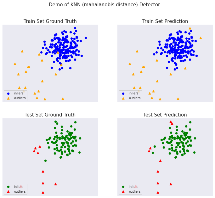
総ての examples に含まれる visualize 関数により可視化を生成します :

from pyod.utils.example import visualize
 
visualize(clf_name, X_train, y_train, X_test, y_test, y_train_pred,
          y_test_pred, show_figure=True, save_figure=False)

以上

タグ: PyOD 0.8

異常検知外れ値検知 & 時系列予測

PyOD 0.8 : Examples : k 近傍法 & マハラノビス距離

PyOD 0.8 : Examples : k 近傍法 & マハラノビス距離

合成データの生成と可視化

モデル訓練

予測と評価

マハラノビス距離

ClassCat® Chatbot

人工知能開発支援

最近の投稿

カテゴリー

異常検知 外れ値検知 & 時系列予測

PyOD 0.8 : Examples : k 近傍法 & マハラノビス距離

PyOD 0.8 : Examples : k 近傍法 & マハラノビス距離

合成データの生成と可視化

モデル訓練

予測と評価

マハラノビス距離

ClassCat® Chatbot

人工知能開発支援

最近の投稿

カテゴリー

タグ

異常検知外れ値検知 & 時系列予測